Show the code
p <- seq(0, 1, 0.01)
v_p <- p * (1 - p)
plot(x = p, y = v_p, type = "l")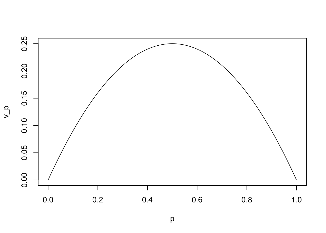
The probability of winning Lotto Max is:
The probability of matching 6 out of 7 numbers is:
\[ \dfrac{(\text{Choose 6 out of 7 correct numbers})\cdot(\text{Choose 1 out of 42 incorrect numbers})}{\text{Choose 7 out of 49 numbers}} \]
For any number \(k\) (between 0 and 7), the probability of matching \(k\) numbers is:
Continuing with the lottery, we have:
We’ve already calculated P(all 7 matches) and P(6 outta 7 matches). To calculate P(5 or fewer matches), we note that:
The expectation (mean) can be found as follows:
If you played the lottery millions of times, you can expect to lose $0.82 each time. Even if you win the jackpot, you’ll still end up losing money if you play enough times!
For a Bernoulli R.V., the variance is p(1-p). When is the variance as high as possible?
Here’s what the plot looks like for all possible values of p:
p <- seq(0, 1, 0.01)
v_p <- p * (1 - p)
plot(x = p, y = v_p, type = "l")
The binomial distribution formula can be inputted directly into R.
For the lecture notes, we need \(P(X = 0)\) where \(X \sim Binom(0.02, 52)\):
However, R is a statistical programming language. Of course it has distributions built in! The distribution function always starts with the letter d.
The cumulative distribution function is also very useful. In R, the cumulative distribution functions always start with a p.
Note that \(P(X \ge 3) = 1 - P(X \le 2)\). We’ll first calculate \(P(X \le 2)\):
And so the answer is:
The following code will help with the card drawing example as well as the expected lottery winnings.