
3 Discrete Distribution Functions
3.1 Binomial Distribution
The binomial distribution formula can be inputted directly into R.
For the lecture notes, we need \(P(X = 0)\) where \(X \sim Binom(0.02, 52)\):
However, R is a statistical programming language. Of course it has distributions built in! The distribution function always starts with the letter d.
Probability Distributions are the
d* series of functions.
dbinom(x = x, size = n, prob = p) calculates \(P(X = x)\), where \(X \sim Binom(n, p)\).
The cumulative distribution function is also very useful. In R, the cumulative distribution functions always start with a p.
Note that \(P(X \ge 3) = 1 - P(X \le 2)\). We’ll first calculate \(P(X \le 2)\):
And so the answer is:
Cumulative Distribution Functions (CDFs) are the
p* series of functions
pbinom(q = x, size = n, prob = p) calculates \(P(X \le x)\), where \(X \sim Binom(n, p)\).
The question above found \(P(X \ge 3)\) is approximately 8%. What if we were given that \(P(X \le q)\) is equal to \(p\) (where \(p\) is given), how would we find \(q\)?
Let’s go back to the coin flipping example. Suppose now we’re flipping 50 coins. We expect that 50% of the time, we’ll get 25 or fewer heads. That is, \(P(X \le 25) = 0.5\). How many heads do we need to flip in order for \(P(X \le x)\) to be equal to 25%?
Inverse CDFs are the
q* family of functions
qbinom(p = p, size = n, prob = prob) finds \(q\) in the equation \(P(X \le q) = p\) when \(X\sim Binom(size, prob)\).
For discrete distributions, there are finitely many probabilities and therefore there may not be an exact value of \(q\) to make the equation true.
In the double check, we see that \(P(X \le 47)\) is actually equal to 33%?!?! Why is this? Let’s see what happens if we check the next number down.
The probability that X is less than 22 is less than 25%. By convention, The inverse CDF is a function that finds the value \(q\) such that \(P(X \le q)\) is at least \(p\). This is easier to see in the plot of the cdf:
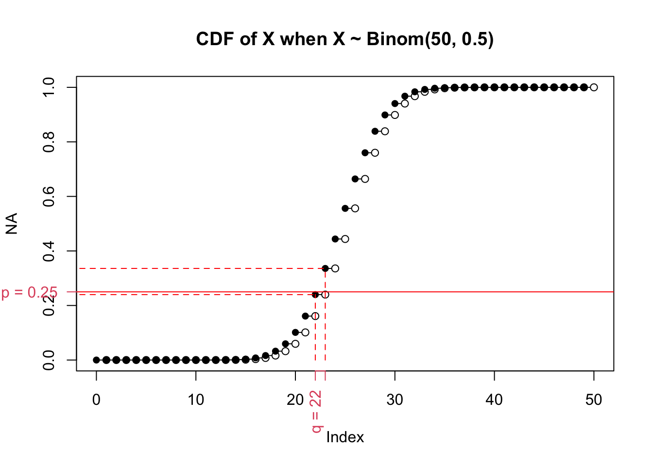
There’s clearly no place where the cdf is equal to 0.25. Instead, we could choose either 0.24 (\(P(X \le 22)\)) or 0.33 (\(P(X \le 23)\)). It might seem convenient to take the closest point, but mathematicians always prefer consistency. In this case, consistency means always rounding up.
Hypergeometric Distribution
Just like the binomial distribution, R has the hypergeometric distribution built into it. dbinom() needed the size and the probability, whereas dhyper() needs the parameters:
m= number of successes (\(a\) in our notation)n= number of failures (\(N - a\) in our notation)k= number of things chosen (\(n\) in our notation)
Note that we’ve already done a hypergeometic problem - the lottery example! Copied from above, let’s choose 6 winning numbers out of 7 possible successes and 49 total things to choose from:
Probability Distributions are the
d* series of functions.
dhyper(x = x, m = a, n = N - a, k = n) calculates \(P(X = k)\), where \(X \sim Hyper(n, a, N)\).
For example 2.4.2: We want the probability that no more than 1 container has trace amounts of benzene, i.e. we want \(P(X = 0) + P(X = 1)\), or equivalently \(P(X \le 1)\).
Cumulative Distribution Functions are the
p* series of functions
phyper(q = x, m = a, n = N - a, k = n) calculates \(P(X \le x)\), where \(X \sim Hyper(n, a, N)\).
As noted in the slides, \(n\) is much smaller than \(N\), so the replacement has very little affect on the answer. If instead we were choosing 10 things out of 10000 with probability of success \(a / N\), then we have \(X \sim Binom(10, 1000/10000)\):
This number is very very close! In general, if we’re sampling a small portion of our potential space, then replacement has a very small effect.