library(ggplot2) # if this fails, run install.packages("ggplot2")
shiny::runGitHub(repo = "DB7-CourseNotes/TeachingApps",
subdir = "Tools/samplingDist")8 Sampling Distributions
Please pay attention to the notes.1 They often contain important information.2
8.1 Prelude: Populations and Samples
The main idea in the rest of the course is this: We can use a sample to say something about the population. Before we dive into that idea, let’s make a distinction.
- Statistic: A number that we calculate from data.
- Population parameter: The value of a statistic if it were calculated for the whole population.
- Sample Statistic: The value of a statistic if it were calculated for a single sample.
For example, we find the mean by taking all of the values and adding them up, then dividing by the number of things we added. For heights of Canadians, the population parameter is the value we would get if we found every Canadians’ height and added them up, then divided by the population of Canada. We obviously can’t do this, but it’s useful to think about. The sample mean is the mean we get when we just have a sample. Since we can only get a sample, it would be super cool if we could use that sample mean to talk about what values of the population mean were reasonable guesses.
In the height example, the population was all Canadians. This isn’t always how we define the population! For example, if we wanted to know the average length of pregnancy, we’d be looking at a population of all people who get pregnant at some point in their lives.
8.2 Introduction
You take a sample. You find the sample mean. Is this mean exactly equal to the population mean?3 Probably not.
Wait, did I just say probably not? How probably? We’ve done a few lectures on probability, so we can probably describe the distribution somehow. What is the probability that the sample mean is within one standard deviation of the population mean? Two standard deviations?
Because of random sampling error,4 every sample is going to have a different mean. We expect most of the sample means to be close to the population mean, with fewer samples resulting in sample means that are further away. In other words, the sample mean should be close to the population mean, but due to sampling error there will be a little bit of a difference.
The variation within our sample should be similar to the variation within the population5, and the variance in the population tells us the variance in the sample means. Variation is not something to be afraid of, and sampling errors are not sampling mistakes; we can harness the variability within a sample to draw conclusions about the population!
8.3 Sampling distribution of the sample mean
Because the value of a sample mean is random (since we took a random sample), there’s a probability distribution that describes it. I could just jump to the answer, but it’s best if I build up to it.
The app below6 will take a random sample from the population (in this case, normal), then find the mean and add it to a histogram. As you collect more means, the histogram gets more and more data. This simulates taking many many different samples.
Play around yourself! Start with \(n\) equal to 2 or 3. The sample shows the individual values, but it also shows the sample mean. Notice how the mean is usually closer to the population mean than any of the individual sample values.
Now, take another sample! Again, the sample mean is closer to the population mean than most of the sampled values. Take more samples. Take 1000 more samples. Notice how the distribution of sample means is bell-shaped, but slightly skinnier than the population.
Repeat what you did above, but use n = 25 or so. The histogram of sample means is even skinnier now! It’s still centered on the population mean, though!
These histograms are approximations to the sampling distribution of the sample mean. If you take an infinite number of samples and calculate the mean for each different sample, you’ll get a distribution of all possible sample means. This is what a sampling distribution is. I’m going to repeat that, since this is often a very difficult topic: the population distribution shows you the probability distribution for all possible individuals, while a sampling distribution shows you the probability distribution for all possible sample means. Each sample has a different mean, the sampling distribution describes many many samples.
8.4 Normal Populations
If the population is normal with mean \(\mu\) and standard deviation \(\sigma\), then there is some relatively straightforward math7 to show that:
\[ \bar X \sim N\left(\mu, \frac{\sigma}{\sqrt{n}}\right) \]
That is, the distribution of all possible sample means8 is normal with the same mean as the population, but with a smaller standard deviation. Go back to the app and see this for yourself.
Example
Suppose the population of heights of Canadian women is N(162.3, 7.11).9 We’re going to try and build up some intuition for why the distribution of all means has a smaller variance than the distribution of the population.
- The probability that a randomly chosen woman is taller than 170 cm is \(P(X > 170)\) =
1 - pnorm(q = 170, mean = 162.3, sd = 7.11)= 0.139. So there’s about a 14% chance of finding a woman taller than 170 cm. - (This is just for example - this part is not often important.10) If we take a sample of n=2 women, what’s the probability that both of them are taller than 170cm? If it’s a truly random sample, then the heights of the two women should be independent and we can just multiply their probabilities.11 This means that there’s approximately \(0.14*0.14 = 0.0193 = 1.93\%\) chance of this. Obviously, if one woman taller than 170 is unlikely, then both women taller than 170 is very unlikely.
- If we take a sample of \(n=2\) women, what’s the probability that their average height is larger than 170? From above, we know that the distribution of the sample mean is \(N(162.3, 7.11/\sqrt{2})\), so we can calculate this probability as \(P(\bar X > 170)\) =
1 - pnorm(q = 170, mean = 162.3, sd = 7.11/sqrt(2))= 0.06. This is somewhere in between just one of them being taller than 170cm and both of them being taller than 170.
When we took a sample of 2 women, one might have been taller than 170 but one might have been shorter, so the average ends up being less than 170. The sample mean is less variable than the individual values, so it’s less likely to be further away.12
Summary
If you take two values from a normal distribution, the average of those two values is probably closer to the true mean than either of the individual values. If you found the average of 100 observations from a normal distribution, the mean of all of those means is probably even closer to the true mean. If you took 200 observations, the mean of means will be even closer!
8.5 Non-Normal Populations with Large Sample Size
In the previous example, we saw that a normal population distribution will result in a distribution for all possible sample means that is also normal, but with a smaller variance. If the population isn’t normal, but you have a large enough sample size, the sampling distribution is still normal. It’s kind of amazing, but it seems to work in practice!
The app below13 will help you understand this relationship. I use an “Exponential distribution” for the population, but this isn’t a distribution you really need to worry about. All you need to know is that the population clearly isn’t normal.
shiny::runGitHub(repo = "DB7-CourseNotes/TeachingApps",
    subdir = "Tools/nLarge")
Regardless of “lambda”14, as n increase, the sampling distribution becomes closer and closer to the normal distribution. By around n=30 or 40,15 they’re basically the same!16
Again,
\[ \text{If }X\sim N(\mu, \sigma)\text{ and n is ``large'', then }\bar X\sim N(\mu,\sigma/\sqrt{n}) \]
where 60 is definitely “large”, 50 is probably “large”, 30 is debatably “large” (depending on what textbook you read), and anything less than 30 is definitely small. I will not test you on the grey areas here.
This result has a very special name:
The Central Limit Theorem
Given a simple random sample of size \(n\) (where \(n\) is “large”) from any population with mean \(\mu\) and standard deviation \(\sigma\), the sampling distribution of the sample mean will follow a \(N(\mu, \sigma/\sqrt{n})\) distribution.
For a perfectly normal population, this is true for any \(n\). For a population that just a little bit not normal, \(n\) must be moderately large. For a very not normal population (e.g. Binomial with \(p\) far from 0.5), we need \(n\) even larger. Still, as long as the sd of the population is finite, the sampling distribution will be normal for sufficiently large \(n\)!
Examples
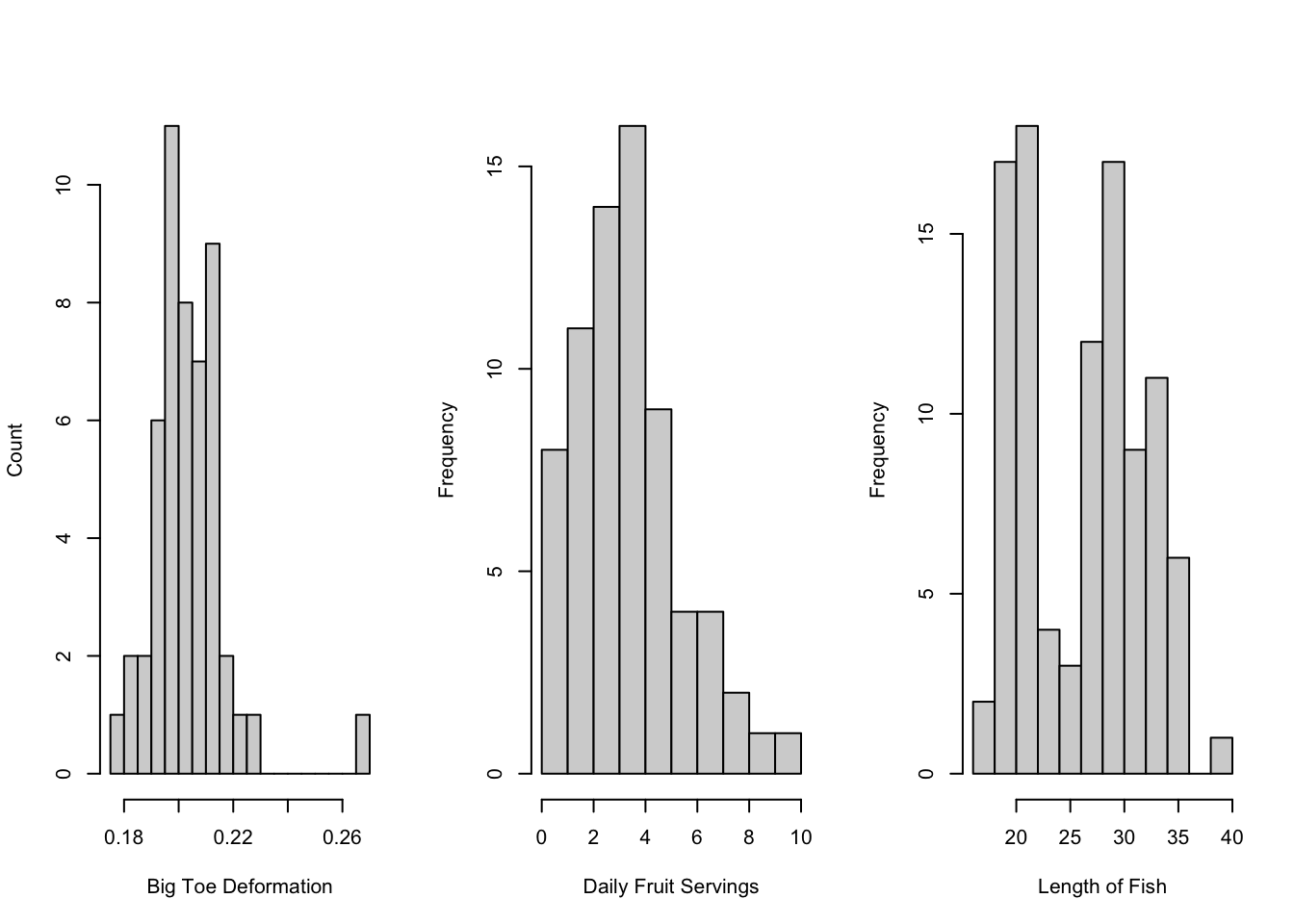
- The angle of big toe deformation in 38 patients.
- There’s an outlier, but the sampling distribution would still be normal even for relatively small \(n\).
- The number of servings of fruit per day for 74 adolescent girls.
- The distribution is clearly (right or left???) skewed17. This makes sense - the number of fruits can only be as low as 0 and there may be many people who don’t eat a lot of fruit, but there will be a few eating many fruits per day!
- The skewness of the data implies skewness in the population (assuming this is a good sample). No worries, though, the sampling distribution will still be normal! We just might need a larger sample size in future studies.
- The lengths of 56 perch from a Swedish lake.
- This is clearly a bimodal distribution, indicating that there might be two subgroups in these data.
- The sampling distribution will still be normal (unimodal), but the mean of this sampling distribution will probably be somewhere in between the two peaks. In other words, it won’t be describing either of the apparent subgroups! No amount of beautiful theorems will ever fix errors in sampling.
- In this case, we would want to find out why there are two subgroups before trying to say anything about the population distributions. If we actually have two types of fish, it’s better to study them separately!
Non-Normal Population with Small Sample Size
This is modelled with the \(t\)-distribution, which will be covered later.
8.6 Very Non-Normal: The Binomial Distribution
Here’s some mild deja-vu:
You roll a dice. You find the sample proportion of heads, denoted \(\hat p\).18 Is this proportion exactly equal to the population proportion? Probably not.
Wait, did I just say probably not? How probably? What is the probability that the sample proportion is within one standard deviation of the population proportion? Yeah, we’re back on this again.
Aside: The normal approximation to Binomial
Most textbooks provide the rule: if both np and n(1-p) are larger than 1019, then the normal distribution is a good approximation to the binomial distribution. I prefer to let you see whether these rules make sense. The app below lets you change n and p, and shows a \(B(n, p)\) and an \(N(np, \sqrt{np(1-p)})\)20 distribution.
shiny::runGitHub(repo = "DB7-CourseNotes/TeachingApps",
    subdir = "Apps/normBinom")
Set n = 20 and find p such that np < 10. Also find p such that n(1-p) < 10. What is the shape of the Binomial distribution in these cases? What do you notice about the normal distribution? Why do both np and n(1-p) need to be greater than 10?21
Binomial? More like Binormial!
It turns out that, with large \(n\) the sampling distribution of \(p\) also follows a normal distribution!22 Even though the population distribution isn’t even continuous,23 the normal distribution approximates it well when there are lots of samples.
For each sample, the actual proportion that you calculate is variable. You might get 3 heads out of 10 flips one time, then 8 heads out of 10 flips the next. On average, though, you’ll get 5 heads out of 10 flips. Formally, the mean of the sampling distribution of the sample proportion is \(p\).24
The variance is a little trickier. In the Binomial lecture notes, I said that the variance increases as n increases. However, when we calculate the proportion, we take the number of successes divided by n. According to some math that is not important for this course, this leads to a variance of the sampling distribution of the sample proportion of p(1-p)/n, which means that the standard deviation25 of the sampling distribution is \(\sqrt{p(1-p)/n}\).
To recap: The variance of a Binomial distribution is \(np(1-p)\). If we take repeated samples from that Binomial distribution and calculate the proportion of sucesses, the variance will be \(p(1-p)/n\).26
Example
Suppose I’m rolling a dice 5 times. The probability of exactly 1 one is defined by the Binomial distribution: dbinom(1, size = 5, prob = 1/6) = 0.4.27 The number of ones we expect after rolling many many dice is \(np = 5/6 =0.8333\). The variance in the number of ones in 5 rolls is \(np(1 - p) = 25/36 = 0.69444\), meaning the standard deviation of the number of ones in 5 rolls is \(\sqrt{np(1-p)} = \sqrt{5/36}\).
Let’s use R to roll some dice for us!
# Rolling 1 dice
# The "r" version of functions givexs random values
# Not on midterm
rbinom(n = 1, size = 5, prob = 1/6)
[1] 1# Rolling 1000 dice
# Not on midterm
dice_1000 <- rbinom(n = 1000, size = 5, prob = 1/6)
mean(dice_1000) # We expect this to be 0.8333[1] 0.834var(dice_1000) # We expect this to be 0.69444[1] 0.7111552The results match! For 1000 rolls of the dice, we got close an average of 0.833 ones per sample (note that this is the number of ones, not a probability). The variance in the number of ones per roll for 1000 is close to the 0.69444 that we expected.
This is the sampling distribution for the number of 1s out of five rolls. However, we generall deal with the probability of a 1 out of 5 rolls.
Exampling Distribution
The following code is not testable - you are not expected to write anything like this. I’m taking repeated samples from a B(75, 0.4) distribution and calculating the proportion of successes for each sample.
set.seed(4)
n <- 75
p <- 0.4

binom_proportions <- c() # empty vector, to be filled later

for(i in 1:1000){ # repeat this 1000 times:
    # This is confusing: I'm getting *one* sample of size n,
    # but R labels the number of samples as n
    new_sample <- rbinom(n = 1, size = n, prob = p)

    # Add the proportion of successes to the vector
    binom_proportions[i] <- new_sample/n
}

hist(binom_proportions,
    breaks = 13, # what happens if you make this larger?
    freq = FALSE) # Divide the heights of bars by the number of obs.
curve(dnorm(x, mean = p, sd = sqrt(p*(1-p)/n)), add = TRUE, col = 3, lwd = 3)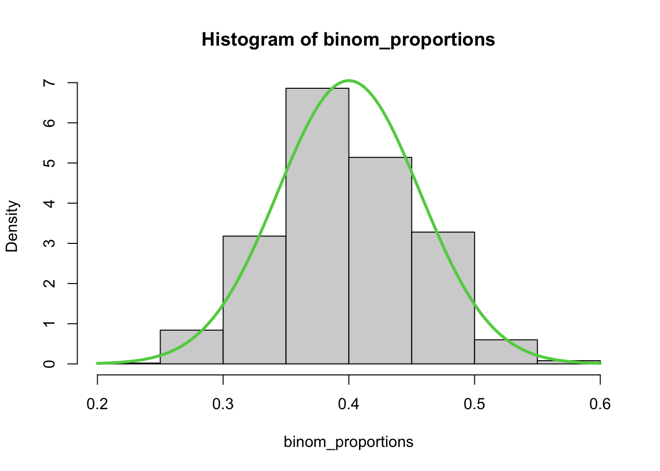
Copy and paste the code above into a script file and observe what happens when you increase the number of breaks. Why does this happen?28
Each sample has a 40% chance to be a success, and this is indeed shown in the sampling distribution. However, due to random sampling, we can get sample proprtions as low as 0.25 and has high as 0.55! Because of randomness, we’ll very rarely (if ever) get a sample value that perfectly matches the population value.
The lesson is this: Even if the true population proportion is 0.4, a sample value of, say, 0.5 is still consistent with the true proportion. This is analogous to saying that the true population mean is 162.3, but our random sample had a mean of 165. The sample value is different from the population value, but still close enough (releative to the variance) to be reasonable.
8.7 Conclusion: Statistics is the Study of Variance
In both of the sampling distributions above, the mean of the sampling distribution was the mean of the population. The difference between the population and the sampling distribution is the variance. In both sampling distributions, the variance decreases as n increases. If you sample the entire population every time you do a sample, there will be no variance in your estimate!
8.8 Self-Study Questions
- When do we use \(N(\mu, \sigma/\sqrt{n})\) versus \(N(\mu, \sigma)\)? When do we use \(N(p, \sqrt{p(1-p)/n})\) versus \(N(np, \sqrt{np(1-p)})\)? This distinction is extremely important.
- If the population is \(N(2,4)\) and we take a sample of size 10, explain why \(\frac{\bar X - 2}{4/\sqrt{10}}\) follows a standard normal distribution. This is extremely important.
- What does it mean for the sample mean to be the same as the population mean? Will they be the same every time you take a sample?
- Play around with the “normBinom” app shown above. Why is the normal distribution not appropriate when np<10 or n(1-p)<10?
- In the “Histogram of binom_proportions”, what happens when you increase the number of breaks? What causes this phenomenon?
8.9 Exercises
For these questions, suppose we know that Candian womens’ heights are normal with a mean of 163cm and a standard deviation of 7cm
- What’s the probability of an individual woman, randomly sampled from the population, being taller than 170 cm?
- What’s the probability that the sample mean is larger than 170cm if:
- \(n = 9\)
- \(n = 16\)
- \(n = 25\)
- What do you notice about the probabilities in question 2?
- Given heights are Normal with a mean of 163 and a standard deviation of 7, what sample size do we need to ensure that 95% of potential sample means are within 2cm of the population mean (that is, 2cm on either side of the mean)?
Answer to Questions 1 and 2
# Question 1
1 - pnorm(170, mean = 163, sd = 7)
[1] 0.1586553# Alternate solution:
# Find the Z-score:
(170 - 163) / 7 [1] 1# A z-score of 1 means that 170 is 1 sd away from the mean
# Probability of being more than 1sd above the mean:
1 - pnorm(1) # Can also use the z-table for pnorm(1)[1] 0.1586553# Question 2
1 - pnorm(170, mean = 163, sd = 7/sqrt(9)) # (a)[1] 0.0013498981 - pnorm(170, mean = 163, sd = 7/sqrt(16)) # (b)[1] 3.167124e-051 - pnorm(170, mean = 163, sd = 7/sqrt(25)) #(c)[1] 2.866516e-07Solution to Question 3
As the sample size increases, the variance decreases (since we’re dividing by the square root of \(n\)). This means that values further away from the mean are less and less likely.
Solution to Question 4
We know that the middle 95% of any normal distribution is within 2 standard deviations of its mean. Because of this, we need 2cm to be equal to 2 standard deviations of the sampling distribution. (Well, technically, it should be -qnorm((1 - 0.95)/2) = 1.96.)
We know that the sample mean will have a normal distribution with a mean of \(\mu\) and a standard deviation of \(\sigma/\sqrt{n}\), so we’re using \(\sigma/\sqrt{n}\) as the standard deviation. Because we don’t have the sample size, we don’t have a value to put into qnorm() and we’ll need to do some math ourselves.
The two paragraphs above tell us that 2cm is equal to 1.96 standard deviations, and the standard deviation of the sampling distribution (the standard error) is \(7/\sqrt{n}\). Setting these equal, we get \(2 = 1.96 *7/\sqrt{n}\) which means \(n = (1.96 * 7/2)^2 = 47.0596\).
We’re not done yet! We can’t sample 47.0596 people! We want to be within two standard deviations of the mean, so we want to make sure that when we round, we don’t go above 2cm. Since the variance of the sampling ditribution decreases as \(n\) increase, the confidence interval is smaller when \(n\) is larger. Because of this, we always want to round up. Even if our answer came to 12.0001, we would round up to 48 to get our final answer.
A short version of this solution: Using R or the normal table, the middle 95% is within 1.96 standard deviations of the mean. Since we’re dealing with a sampling distribution, the standard deviation is \(7/\sqrt{n}\). Setting these two numbers equal, we get \(2 = 1.967/\sqrt{n}\) and we solve for \(n\). We round up, because we want our interval to be less than 2cm on either side and because a larger sample has lower variance.
8.10 Crowdsourced Questions
The following questions are added from the Winter 2024 section of ST231 at Wilfrid Laurier University. The students submitted questions for bonus marks, and I have included them here (with permission, and possibly minor modifications).
- What factor primarily contributes to the sampling distribution having a lower variance than the population distribution?
- reduction in standard deviation within the sample
- the wider range of possible values in the population
- utilization of a different statistical methodology for sampling
- summarization of multiple observations into a single value during sampling
Solution
- is the correct answer. When creating a sampling distribution, multiple samples from a population are taken to create a statistic for each sample. As more samples are taken, the statistic will represent the true population parameter better. Essentially, as more values are summarized into one, there is a reduced variability in the sampling distribution compared to the population.
- Let X represent the heights, in metres, of white birch trees in Saskatchewan. Given that it follows a normal distribution with a mean of 8 and a standard deviation of 5, the heights of a randomly selected group of n=6 trees are measured. Find the probability that the sample mean tree height is at most 10 m.
Solution
First, let’s label all of the information we have been provided:
- sample size: \(n = 6\)
- population mean: \(\mu = 8\)
- population stdev: \(\sigma = 5\)
Since there is a sample size of 6 trees, the mean of the sampling distribution will still remain 8 but the standard deviation of the sampling distribution is \(\sigma/\sqrt{n} = 5 / \sqrt{6} = 2.04\)
Since the height can be a maximum of 10m, we are trying to find P(\(\bar x\) < 10). We can find this by standardizing and using the z-table:
P(x6 < 10) = P(Zx6 < (10-8) / 2.04) = P(Zx6 < 0.98) = 0.8365
Therefore, in a sample of 6 trees, there is a 83.65% (or 0.8365) chance that a silver birch tree in Saskatchewan is at most 10 m tall.
In R:
pnorm(10, mean = 8, sd = 5 / sqrt(6))[1] 0.8364066- the scores on a standardized test are normally distributed with a mean of 75 and a standard deviation of 10.
- what percentage of students scored above 85?
- if the top 15% of students receive a special award, what is the minimum score required to receive the award?
- if a random sample of 50 students is selected, what is the probability that the sample mean score is greater than 78?
Solution
- to find the percentage of students who scored above 85, we can use the z-score formula:
where: z = x - μ / σ
x = score
μ=75 (mean)
σ=10 (standard deviation)
calculating the z-score: z=85−75 / 10 =1
by looking at a normal distribution table, we find that the percentage of students who scored above z or 1 was 15.87%
- to find the minimum score required to receive the award (the score corresponding to the top 15%): using the inverse standard normal distribution table or calculator, we find that the z-score corresponding to the top 15% is approximately z=1.04. now, we can use the z-score formula to find the corresponding score: x=μ+z⋅σ
x=75 + 1.04⋅10 = 85.4
- for a random sample of 50 students, we need to use the central limit theorem. since the sample size is large (n > 30), the sample mean will be approximately normally distributed. the mean of the sample distribution will be the same as the population mean (μ=75), and the standard deviation of the sample distribution (σˉ) will be the population standard deviation divided by the square root of the sample size: σˉ= σ / √n = 10 / √50 = 1.41
we calculate the z-score for x=78:
z = 78 - 75 / 1.41 = 2.13
using the standard normal distribution table, we find that the probability of obtaining a z-score greater than 2.12 is approximately 0.017. therefore, the probability that the sample mean score is greater than 78 is approximately 0.017, or 1.7%.
In R:
# a) P(X < q) = pnorm(q), so P(X > q) = 1 - pnorm(q)
1 - pnorm(85, mean = 75, sd = 10)
[1] 0.1586553# b) qnorm calculates the value q such that P(X < q) = p, where p is given.
qnorm(1 - 0.15, mean = 75, sd = 10)[1] 85.36433# c)
1 - pnorm(78, mean = 75, sd = 10 / sqrt(50))[1] 0.01694743- Which of the following best describes the Central Limit Theorem (CLT)?
- The CLT states that as the sample size increases, the sampling distribution of the sample sum approaches a uniform distribution, regardless of the shape of the population distribution.
- The CLT asserts that the sampling distribution of the sample mean will be perfectly normal only if the population distribution is normal.
- The CLT guarantees that for any population with a finite mean and variance, the sampling distribution of the sample mean approaches a normal distribution as the sample size becomes large.
- According to the CLT, the mean of the sampling distribution of the sample mean is always equal to the population mean, regardless of the sample size.
Solution
The correct answer is C) The CLT guarantees that for any population with a finite mean and variance, the sampling distribution of the sample mean approaches a normal distribution as the sample size becomes large.
These things!↩︎
Or silliness.↩︎
Recall: population refers to the population of interest. The population mean is the true mean of the population.↩︎
In statistics, error does not mean mistake.↩︎
Assuming we have a good sample.↩︎
You’ll probably see it in the next stats course you take.↩︎
i.e. the sampling distribution of the sample mean↩︎
Note: these numbers actually come from a sample, and we don’t know that the population is normal. We’re making some massive assumptions here.↩︎
You will not need to do something like this on a test.↩︎
Remember the most important fact from probability: Multiplying probabilities only works when they’re independent.↩︎
Take a moment and make sure you understand this relationship. Write out a description of it. Call a grandparent and try to explain it to them.↩︎
Or the same app as before, with population set to Exponential.↩︎
Which controls how skewed the population distribution is.↩︎
I will either ask you questions where n < 30 (non-normal sampling distr.) or n > 50 (normal sampling distr.), nothing in between.↩︎
Although, in this case, the normal approximation is biased, but the bias decreases as n increases and you’re not expected to know these details.↩︎
Answer: right↩︎
i.e. \(\hat p\) = number of success divided by number of trials.↩︎
Or sometimes 15. Again, I won’t test you on the grey areas.↩︎
Recall that the mean and sd of a Binomial distribution are np and np(1-p), respectively.↩︎
Answers: Skewed; positive probability below 0 or above n; symmetric.↩︎
Again, we use the rule of thumb that \(np>10\) and \(n(1-p)>10\).↩︎
This is important.↩︎
Not n*p, since the proportion of heads is x/n.↩︎
Which is simply the square root of the variance.↩︎
Notice how they’re equal when n = 1. When n=1, we’re just taking individuals from the population and calling each individual a sample.↩︎
In other words, 1 successes in 5 trials, where a success is defined as “rolling a one”.↩︎
Hint: What are the possible values of \(\hat p\)?↩︎