14 Two-Sample t-Tests

Author

Devan Becker

Published

2021-10-07

14.1 How much can one more sample complicate things?

Notation: Subscripts everywhere!

We now have two samples.

$\bar X_1\sim N(\mu_1, \sigma_1/\sqrt{n_1})$, where $s_1$ is the estimated standard deviation of a given sample.

$\bar X_2\sim N(\mu_2, \sigma_2/\sqrt{n_2})$

Goal: Are the means the same? I.e., is $\mu_1 = \mu_2$?

With two samples, the difference in means has a sampling distribution. What is that distribution? It’s difficult!

The easy part is the mean of the difference. The mean of the difference is the difference in means. \[ \bar X_1 - \bar X_2 \sim N(\mu_1 - \mu_2, ???) \]

The hard part is the standard deviation of the difference. Take a moment and think about what we’re talking about here. What does it actually mean for the difference in means to have variance?

It’s the same as it was before, it just seems a little more complicated. When we take a pair of samples then find their difference, we have calculated a statistic! For every pair of samples, we’ll get a different statistic. The variance that we seek is the variance of all of these statistics.

The standard deviation of a difference

Again, I’m going to use a simulation to demonstrate what happens if we take a bunch of pairs of samples, then find their difference.

In this case, I’m sampling x1 as 22 values from a normal distribution with a mean of 0 and a standard deviation of 2, whereas x2 has 33 observations and comes from a distribution with a mean of 0 and a standard deviation of 3. I’m finding their means, then finding their differences. I repeat this 10,000 times, keeping track of what the difference in means was.

## approximating the sampling distribution
differences <- c()
for(i in 1:10000){
    m1 <- mean(rnorm(22, 0, 2))
    m2 <- mean(rnorm(33, 0, 3))
    differences[i] <- m1 - m2
}
sd(differences)

[1] 0.6802144

… it’s not at all obvious where this number comes from.

Both had a mean of 0, so the difference should be 0. But the standard deviation of the differences isn’t obvious. There is a nice formula for the mean - $\sigma/\sqrt{n}$ - but it’s not obvious how this works for two samples with different variances and different sample sizes!

It turns out that the following equation is the correct one for the standard deviation of the differences. Recall that the standard deviation of a sampling distribution is known as the Standard Error (SE).

\[ SE = \sqrt{\frac{s_1^2}{n_1} + \frac{s_2^2}{n_2}} \]

And to verify that our simulation matches this idea:

## Check
sd(differences)

[1] 0.6802144

sqrt(4/22 + 9/33) # Close enough

[1] 0.6741999

Putting it Together

Altogether, this means that the difference between means has the following sampling distribution:

\[ \bar X_1 - \bar X_2 \sim N\left(\mu_1 - \mu_2, \sqrt{\frac{s_1^2}{n_1} + \frac{s_2^2}{n_2}}\right) \]

From this, we get the same general ideas as before. The hypothesis tests are based on the observed test statistic: \[ t_{obs} = \frac{\text{sample statistic} - \text{hypothesized value}}{\text{standard error}} = \frac{(\bar x_1 - \bar x_2) - 0}{\sqrt{\frac{s_1^2}{n_1} + \frac{s_2^2}{n_2}}} \] where usually the hypothesized value is 0 so that we’re testing whether the true population means are the same.

Two-Sample Hypotheses

The usual null hypothesis invloves the equality of the means, with the alternative being “>”, “<”, or “≠”. This does not change: \[\begin{align*} H_0: \mu_1 = \mu_2 &\Leftrightarrow H_0:\mu_1 - \mu_2 = \mu_d = 0\\ H_0: \mu_1 < \mu_2 &\Leftrightarrow H_0:\mu_1 - \mu_2 = \mu_d < 0\\ \end{align*}\]

The confidence interval is also the same idea: \[ \text{sample statistic}\pm\text{critical value}*\text{standard error} = (\bar x_1 - \bar x_2)\pm t^*\sqrt{\frac{s_1^2}{n_1} + \frac{s_2^2}{n_2}} \]

In both of these, we still need to know the degrees of freedom! As we saw last lecture, the $t$-distribution requires some information about the sample size. In the one-sample case, this was $n-1$. However, we now have two potentially different sample sizes! What do we do?

Recall that the $t$-distribution gets closer and closer to the normal distribution as $n$ increases. The whole point of the $t$ is to get us a little further from the normal in order to account for the variance in the sample standard deviation. For the two-sample case, there is a “correct” formula, but it’s big and scary and everything we’re doing now is approximate anyway. Instead, we use a more conservative approach to ensure that we’re not underestimating the variance.¹

Two-Sample $t$ degrees of freedom

When doing hand calculations, we use the smallest sample size, then subtract 1. (R does a more accurate calculation that results in non-integer values.)

In the simulation we did earlier, the two samples had sizes of 22 and 33. In both a CI and a hypothesis test, we would use 21 as the value in qt() or pt() (which are the same idea as qnorm() and pnorm()).

Aside: “Pooled Variance”

There’s another formula out there that uses a so-called “pooled variance” for the standard error of the differences. This assumes that both populations have the exact same variance, and tries to use information from both to estimate the variance. It essentially treats the two samples as one big sample from the same population in order to calculate the standard deviation.

This also implicitly assumes that both populations are normal, and this is not based on the CLT. Instead, the populations need to be normal. This is a huge assumption - we can use normality from the CLT because the math checks out. Assuming normality of the population is just a wild guess that we can’t really check.

It is also very, very unlikely that the two populations have the same standard deviation.

If the two assumptions are met, then the pooled standard deviation is the “correct” formula. However, the SE that we saw before still works very well! If the assumptions are not met, then the pooled SE works poorly and the SE we’ve seen is still very good!

Except in exceptional cases, the SE that we’ve learned should be used. The idea of a pooled variance is a vestige of another age (and may show up if you use another textbook or search Google).

14.2 Summary

Two-Sample t-test and CI Overview

We are usually testing for the difference in means, i.e. \[\begin{align*} H_0: \mu_1 = \mu_2 &\Leftrightarrow H_0:\mu_1 - \mu_2 = \mu_d = 0\\ H_a: \mu_1 < \mu_2 &\Leftrightarrow H_a:\mu_1 - \mu_2 = \mu_d < 0\\ \end{align*}\]

\[ t_{obs} = \frac{\bar x_1 - \bar x_2}{\sqrt{\frac{s_1^2}{n_1} + \frac{s_2^2}{n_2}}} \]

\[ \text{p-value} = P(T < t_{obs}) = \texttt{pt(t\_obs, df = min(n1, n2) - 1)} \]

\[ \text{A $(1-\alpha)$ CI for $\mu_d$ is }\bar x_1 - \bar x_2 \pm t^*\sqrt{\frac{s_1^2}{n_1} + \frac{s_2^2}{n_2}} \]

where $t^*$ is based on the smaller of $n_1 - 1$ and $n_2 - 1$

The assumptions are still the same, with one notable addition:

The sampling distribution of the difference in means is approximately normal.
- Normal populations, approximately normal histograms, or large sample size.
The observations within each group are independent.
The observations between each group are independent.

14.3 Example 1: Two-Sample versus Matched Pairs

From the Ointment example:

	Subject 1	S2	S3	S4	S5	S6	S7	S8
With Oint	6.44	6.06	4.22	3.3	6.5	3.49	7.01	4.22
Without	7.22	6.05	4.55	4	6.7	2.88	7.88	6.32
Difference	-0.78	0.01	-0.33	-0.7	-0.2	0.61	-0.87	-2.1

First we’ll do matched pairs. In this example, this is the correct test to use.

withoint <- c(6.44, 6.06, 4.22, 3.3, 6.5, 3.49, 7.01, 4.22)
without <- c(7.22, 6.05, 4.55, 4, 6.7, 2.88, 7.88, 6.32)
diff <- withoint - without

hist(diff)
abline(v = 0, col = "red", lwd = 2)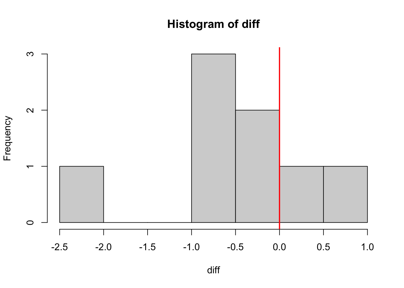

t.test(x = diff, alternative = "less")


    One Sample t-test

data:  diff
t = -1.9421, df = 7, p-value = 0.04663
alternative hypothesis: true mean is less than 0
95 percent confidence interval:
        -Inf -0.01332314
sample estimates:
mean of x 
   -0.545

From this t-test, we can see that there’s a mean difference of -0.545, which leads to a p-value of 0.04663. At the 5% level, the null is rejected and we conclude that there is a difference between the two groups. The ointment appears to make a difference!

However, looking at the histogram, it looks like there may be an outlier. With a data set this small, one value can completely change our results!!! Remember that we’re dealing with means, and means are affected by outliers. This means that p-values are affected by outliers as well!

The Wrong Way

We could instead have done a two-sample test, which ignores the fact that the observations are paired. Since we know the pairings, this test is leaving out valuable information.

boxplot(withoint, without)
abline(v = 0, col = "red", lwd = 2)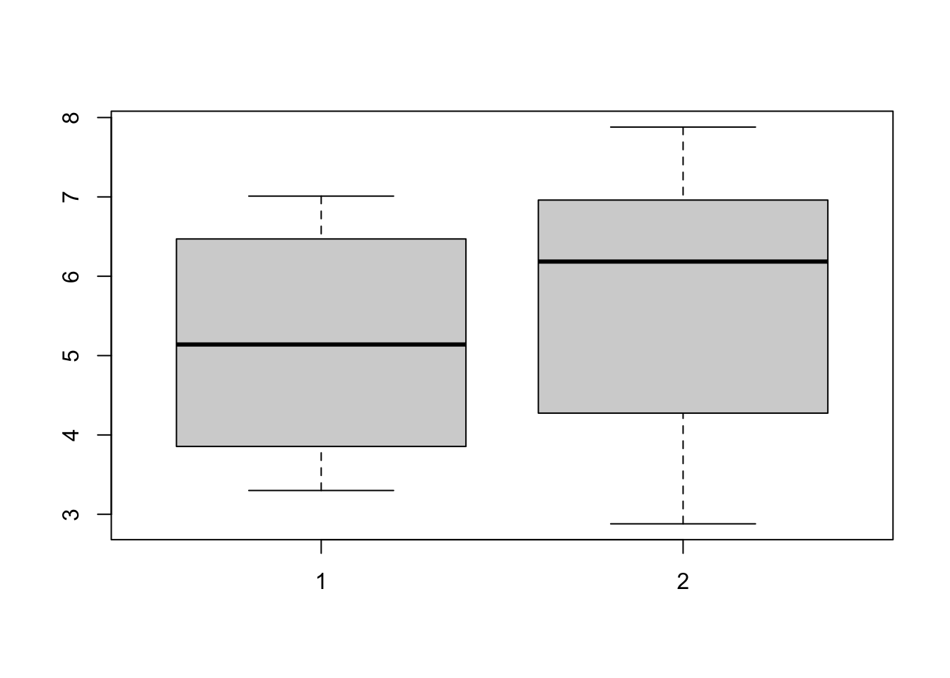

t.test(x = withoint, y = without, alternative = "less")


    Welch Two Sample t-test

data:  withoint and without
t = -0.67584, df = 13.736, p-value = 0.2552
alternative hypothesis: true difference in means is less than 0
95 percent confidence interval:
      -Inf 0.8772719
sample estimates:
mean of x mean of y 
    5.155     5.700

This result should not be trusted since it misses a key aspect of the data. The first value in the “Ointment” group corresponds to the first value in the “Without Ointment” group, they aren’t just two separate values - they’re measured on the same individual!

Regardless, take a moment to look at the differences in the results between the two tests.

14.4 Example 2: Body Mass of Penguins

In this example, we’ll look at the difference in body mass between male and female penguins.

In this case, there is no clear pairing between the penguins. If they were monogomous couples, then the differences in body mass might tell us about couples, but doesn’t say much about male and female penguins in general.²

This example gives us the opportunity to learn more notation in R! The previous example used t.test(x = ..., y = ...) to denote the two samples. If the data are neatly formatted in a data frame, then we can use the ~ notation to demonstrate that the body mass is split into different groups for male and female.

First, we’ll draw a boxplot. This is a great way to compare two distributions, and can be made in a small amount of space. Pause for a moment and ask yourself whether these two groups intuitively look different.

library(palmerpenguins)
boxplot(body_mass_g ~ sex, data = penguins, horizontal = TRUE,
    xlab = "Body Mass (grams)", ylab = NULL)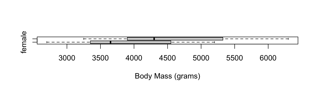

t.test(body_mass_g ~ sex, data = penguins)


    Welch Two Sample t-test

data:  body_mass_g by sex
t = -8.5545, df = 323.9, p-value = 4.794e-16
alternative hypothesis: true difference in means between group female and group male is not equal to 0
95 percent confidence interval:
 -840.5783 -526.2453
sample estimates:
mean in group female   mean in group male 
            3862.273             4545.685

Note: The notation will always be “variable we care most about” ~ “other variables”. In linear regression, this was y ~ x, and now it’s continuous ~ categorical.

From the output above, we get a two-sided p-value as well as a two-sided CI, both confirming that the difference in body mass is different from 0. You can also see that it’s using “female minus male”, rather than “male minus female”. This is because R will put them in alphabetical order, so female comes first.

You may also be happy to hear that no, you will never have to manually enter the standard error formula! Let’s all say a big, collective thank you to the R programming language! Thank you! (You may need to interpret the idea of standard error in two-sample t-tests, though.)

14.5 Example 3: Birthweights (by hand)

Do mothers who smoke give birth to children with a lower birthweight than mothers who don’t?

Test this at the 5% level using the data on the right.

We’re going to do this by hand!

	Smoker	Non-Smoker
mean	6.78	7.18
sd	1.43	1.60
n	50	100

The null hypothesis is $H_0: \mu_{smoke} = \mu_{non}$, which can be written as $H_0: \mu_{non} - \mu_{smoke} = 0$.
The alternate hypothesis is $H_a: \mu_{smoke} < \mu_{non}$, which could be written as
- $H_a: \mu_{non} - \mu_{smoke} > 0$, or
- $H_a: \mu_{smoke} - \mu_{non} < 0$

It doesn’t matter which we choose, but we have to know which we chose in order to calculate the corresponding p-value! Let’s use $\mu_{n-s}$.

The sample mean difference is $\bar x_{non} - \bar x_{smoke} = 7.18 - 6.78 = 0.4$. The standard error is: \[ SE = \sqrt{\dfrac{s_s^2}{n_s} + \dfrac{s_n^2}{n_n}} = \sqrt{\dfrac{1.43^2}{50} + \dfrac{1.60^2}{100}} = 0.2578721 \]

Since we used $\bar x_{non} - \bar x_{smoke}$, our alternate tells us to find the p-value for a t-statistic larger than what we got.

\[ t_{obs} = \dfrac{(\bar x_{non} - \bar x_{smoke}) - (\mu_{non} - \mu_{smoke})}{SE} = \dfrac{0.4 - 0}{0.2578721} = 1.55 \]

Since we’re doing a right-tailed test³, we calculate our p-value as:

1 - pt(1.55, 49)

[1] 0.06378844

To summarise:

$H_0: \mu_{non} - \mu_{smoke} = 0$ versus $H_0: \mu_{non} - \mu_{smoke} > 0$
$t_{obs} = 1.55$
p-value is 0.06

Since our p-value is larger than 0.5, we do not have a statistically significant result. We fail to reject the hypothesis that smokers have lower birthweights. We conclude that we do not have enough evidence to say that smoking is associated with lower birthweights.

14.6 Example 4: Basketball versus Hockey Players

In a previous lecture, we looked at the heights of female basketball players to test whether their heights were consistent with the population. Now that we have the tools to compare two samples, let’s compare some teams! In what follows, we’re testing the the hypothesis that the basketball team and the hockey team are different heights. Let’s test at the 5% level since we have no strong reason to use a smaller or larger level⁴

library(dplyr)
library(ggplot2)
stats <- read.csv("wlu_female_athletes.csv")
baskey <- filter(stats, Sport %in% c("Hockey", "Basketball"))
boxplot(Height ~ Sport, data = baskey)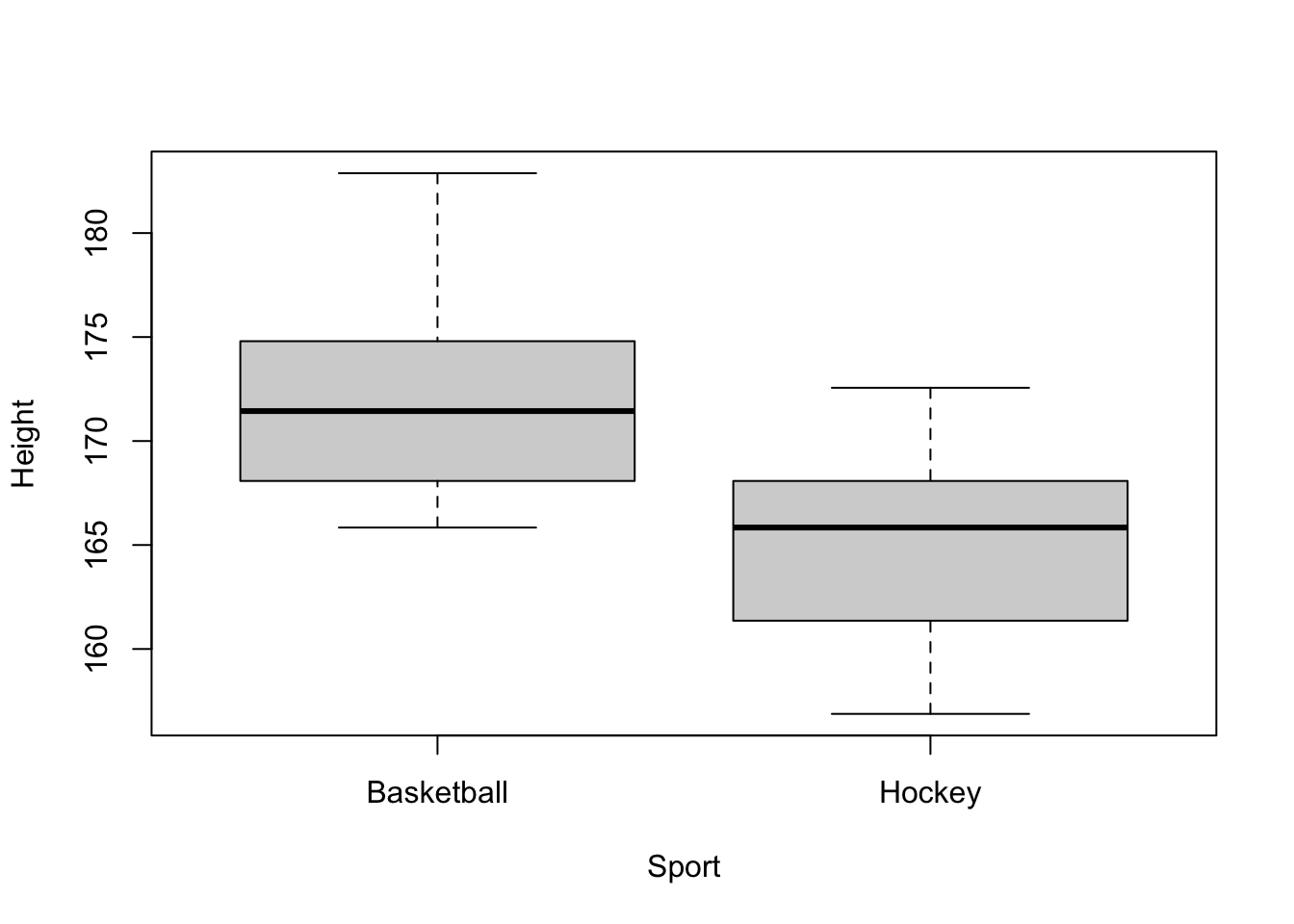

From the boxplot, I would be absolutely flabbergasted if the two groups had the same mean! Astonished! Befuddled, even! This is an important part of any analysis: have expectations! You should know your data well before diving into a study. For example, looking at these boxplots reveals that there are no apparent outliers, and both groups look approximately symmetric. This is good.

Let’s do the t-test.

t.test(Height ~ Sport, data = baskey)


    Welch Two Sample t-test

data:  Height by Sport
t = 4.5266, df = 26.588, p-value = 0.0001121
alternative hypothesis: true difference in means between group Basketball and group Hockey is not equal to 0
95 percent confidence interval:
  3.805256 10.123430
sample estimates:
mean in group Basketball     mean in group Hockey 
                172.1771                 165.2128

From the output, we can conclude that there is a statistically significant difference in the average height of female hockey and basketball players at Laurier.

Some caveats:

These are small samples!!!
- Recall that R uses a more accurate value for df (we just use the smaller sample size then subtract one for hand calculations). It’s 26.588, which can be interpreted as something like the average of the two sample sizes.
This isn’t exactly a random sample!
- The data were taken from the current seasons’ full teams. We don’t exactly have a wel–defined population here. Is the population all women? Only femal athletes? Only female varsity athletes? Only Canadian female varsity athletes in these particular sports? Or is it only female varsity athletes in these particular sports at Laurier? It’s hard to say what these results apply to.
We just tested hockey versus basketball. What about soccer? What about heights by position?
- If we start testing many hypotheses, we run afoul of the multiple comparisons problem. Before collecting the data, this test had a 5% chance of being significant if the null hypothesis were true. So do all of the other tests. If we test enough times, we’ll eventually reject a true null hypothesis.

14.7 Conclusion

If you can have matched pairs, you should use a matched pairs test.
Most of the time, you’ll need to use a two-sample t-test.
- Don’t get fooled by equal sample sizes! Just because the sample sizes are the same doesn’t mean that the observations are paired!
A two-sample t-test is based on the difference in means
- The standard error is tricky - software will do this for you.
- The degrees of freedom is the smallest sample size minus 1.
  - Used for the p-value for hypothesis tests and the critical value for confidence intervals.
  - R uses a better value.
- The null hypothesis is usually 0, and the alternate depends on the order in which you subtract the means.

14.8 Self-Study Questions

Write out the null and alternate hypotheses for the “Ointment” example and the “Penguins” example, and comment on the difference between the two examples. Make sure the alternate has the same “>” or “<” or “≠” that was used in R’s calculation! Hint: It matters if you do Group 1 minus Group 2 or if you do Group 2 minus Group 1!
Veryify the p-values in the Ointment and Penguins examples. Use the t-value reported in the R output, and find the p-value using either pt(), 1 - pt, or 2 * (1 - pt()), as appropriate. Explain your answer.
Explain why t-tests can only be used for comparing two groups, not three. (Hint: write out the null hypothesis - what value are we using in $\mu = \mu_0$?)
Explain why the 95% CI still has the same interpretation as before.
Explain why there is only one sampling distribution in a two-sample t-test, even though there are two populations.
Provide a conclusion based on the following output (suppose you’re testing at the 10% level). The mpg variable is the miles per gallon of a vehicle, while am is the transmission type, with 0 = Automatic and 1 = Manual. mtcars is just the name of the data that these variables are in.

t.test(mpg ~ am, data = mtcars)


    Welch Two Sample t-test

data:  mpg by am
t = -3.7671, df = 18.332, p-value = 0.001374
alternative hypothesis: true difference in means between group 0 and group 1 is not equal to 0
95 percent confidence interval:
 -11.280194  -3.209684
sample estimates:
mean in group 0 mean in group 1 
       17.14737        24.39231

Selected Solutions

Ointment: $H_0: \mu_{without-with} = 0$ versus and $H_A: \mu_{without-with} < 0$. Note that we can tell that it’s without-with by looking at the means of the two groups and the sign of the t-statistic.
- Penguins: $H_0: \mu_{female} - \mu_{male} = 0$ versus $H_A: \mu_{female} - \mu_{male} \ne 0$.
- The ointment example had $\mu_{without - with}$ as a single number, whereas the penguins example used $\mu_{female} - \mu_{male}$, which is the difference between two numbers. This is because the ointment example was a one-sample t-test since we were treating the set of differences as a single sample; the penguins example is a two-sample t-test.

14.9 Crowdsourced Questions

The following questions are added from the Winter 2024 section of ST231 at Wilfrid Laurier University. The students submitted questions for bonus marks, and I have included them here (with permission, and possibly minor modifications).

A biologist is comparing the mean heights of two species of plants. Species A has a sample mean height of 15 cm with a standard deviation of 2 cm from a sample of 30 plants. Species B has a sample mean height of 17 cm with a standard deviation of 3 cm from a sample of 35 plants. What does the two-sample t-test assess in this scenario?
1. Whether the sample means of Species A and Species B come from populations with the same variance.
2. Whether the mean height of Species A is greater than the mean height of Species B.
3. Whether there is a significant difference between the population means of the two species.
4. Whether the combined mean height of both species exceeds a specific value.

Solution

C; The two-sample t-test in this scenario assesses whether there is a significant difference between the population means of Species A and Species B. It does not test for variance equality, the direction of the difference (unless specified as a one-tailed test), or any specific value exceeding the combined means.

A researcher conducts an experiment to determine if there will be a significant difference in the growth rate of two different species of plants under identical laboratory conditions. The first group of 20 plants (Species A) showed an average growth of 5 cm over a month, while over the same period of time the second group of 20 plants (Species B) showed an average growth of 6 cm. Assume the growth rates follow a normal distribution. explain what steps you would take to determine if the observed difference is statistically significant. Consider a 5% significance level for your decision.