Now that we’ve covered the basics of confidence intervals and p-values, there is a huge world of inference to explore! What follows is a small window into the cautions and best practices of inference, especially with regards to p-values.
11.1 Interpreting p-values
A p-value is the probability of a result that is at least as extreme as the one we observed, given that the null hypothesis is true.
It’s a measure of evidence against the null. We assume that the null is true, then ask how likely our sample would be. There isn’t a problem with our sample, so if it’s unlikely then it must be our assumption that is wrong.
“Given that the null hypothesis is true”
Any interpretation of a p-value that does not assume that the null hypothesis is true is a bad interpretation.
The following interpretations are not valid:
The probability of getting data like this.
Probability of our data by chance alone.
Would be correct if we made reference to the null
The probability that the null hypothesis is true
This is just so wrong, but it unfortunately appears in a lot of published papers.
Always look for wording that assumes that the null is true, and searches for evidence against it.
11.2 Statistical Versus Practical Significance
Suppose a new drug claims to increase your lifespan significantly. Wow! That sounds great!
After hearing this claim, you dig into the paper that made the claim, and found that the drug increases the average lifespan by 3 hours. How can they claim this was significant???
This is the difference between statistical and practical significance. The probability of a result at least as extreme, given that the null hypothesis is true, says nothing of how extreme the results are. A very small effect size can be statistically significant, even if it’s not a noticable change in practice.
Furthermore, maybe this new drug costs $1,000 per day and has intense nausea as a side-effect. A statistically significant difference says absolutely nothing about the practical effects.
p-values were never meant to be the goal of a study.
They are yet another tool in the health researcher’s repertoire, meant to test whether data provide enough evidence against a very particular hypothesis.
11.3 Choosing a Significance Level
To build intuition, we start from the extremes:
A significance level of \(\alpha = 0\) will never reject the null hypothesis.
No amount of evidence will convince you.
A siginficance level of \(\alpha = 1\) will always reject the null hypothesis.
Any evidence will convince you.
When setting a confidence level, you must consider how much evidence you require. To quote Carl Sagan: “Extraordinary claims require extraordinary evidence.”
Here are some examples:
A new cancer treatment costs 10 times as much and the patient will never heal back to 100% health. To justify such a procedure, we want to be reeeeeaaaaalllly sure that it works, so we might set a significance level of \(\alpha=0.001\) before we collect any data.
We are making a slight change to an advertising strategy that is based on scientific evidence. We’re fairly certain it will work, and the consequences of it not working are very small. A larger significance level, perhaps \(\alpha = 0.1\), might be appropriate.
\(\alpha = 0.1\) is probably the largest significance level you will ever encounter.
👽 Aliens example: There’s an abberation in an image taken by a digital camera. According to the manufacturer, such an abberation would occur in 0.0001% of the pictures. If we think it’s aliens, that’s an extraordinary claim! We’d need some very strong evidence. Do you think that 0.0001% is strong enough? (We’ll return to this later in the chapter.)
11.4 Hypothesis Errors
When you test a hypothesis, there are two types of errors: You could reject when the null is true or you could fail to reject when the null is false. The following matrix summarises this:
H_0 is TRUE
H_0 is FALSE
Don’t Reject
Good!
Type 2 Error
Reject
Type 1 Error
Good!
In other words:
Type 1: False Positive
Type 2: False Negative
There’s another important point here: rejecting the null hypothesis does not mean that it’s actually false! Any number of things might have happened, such as including an outlier or taking a biased sample.
Similarly, failing to reject a null does not mean that it’s true. We’ve already talked about this a bit - confidence intervals are all values that would not be rejected by a hypothesis test, so there are many plausible null hypotheses! However, we can also fail to reject the null even though it’s false. This can also happen for multiple reasons:
Sample size is too small.
The distance between the null and the sample mean is calculated relative to the standard error. The standard error decreases with a larger sample, so if our sample isn’t big enough then we might not have collected enough evidence to reject the null, regardless of whether it’s true.
Large variability in the data.
This is the other thing that can increase the standard error. With more variation, the distance between the null and the sample mean doesn’t seem as large!
We can fix this with better sampling strategies and with better study designs, or by getting a larger sample size!
Our significance level is too high.
This isn’t really something that we can change after we’ve seen the data.1
The Probability of Type 1 Errors
What’s the probability your reject the null, even though it’s true? Let’s say we reject the null if the p-value is, say, less than 5%. This means that any value in the 5% tails of the distribution would lead to us rejecting the null hypothesis - even though it’s true!2 The probability that we do this is 5%, since there’s a 5% chance that we’ll see a value that is “too unlikey” at the 5% level.
As usual, I like to demonstrate things via simulation. Here’s the setup:
Set the population parameters as \(\mu = 0\) and \(\sigma = 1\)
Simulate normal data
Do a two sided test for \(H_0: \mu = 0\)
Note that this null hypothesis is TRUE
Count how many times we reject the null.
set.seed(21); par(mar =c(2,2,1,1)) # unimportant## set an empty vector, to be filled with p-valuespvals <-c() for(i in1:10000){ # repeat 10,000 times# Simulate 30 normal values with a population mean of 0 and sd of 1 newsample <-rnorm(n =30, mean =0, sd =1)# Test whether the population mean is 0 newsample_mean <-mean(newsample) newsample_sd <-1/sqrt(30) # Assuming population sd is known my_z_test <-2* (1-pnorm(abs(newsample_mean), mean =0, sd = newsample_sd))# record the p-value (the output of t.test has some hidden values) pvals[i] <- my_z_test}## Testing at the 5% levelsum(pvals <0.05) /length(pvals) # should be close to 0.05
[1] 0.0481
Since we’re testing at the 5% level, this value is close to 5%! It’s a little tricky to get your head around: If we think 5% is too unlikely, then we reject the null. However, things that have “only” a 5% chance happen about 5% of the time!
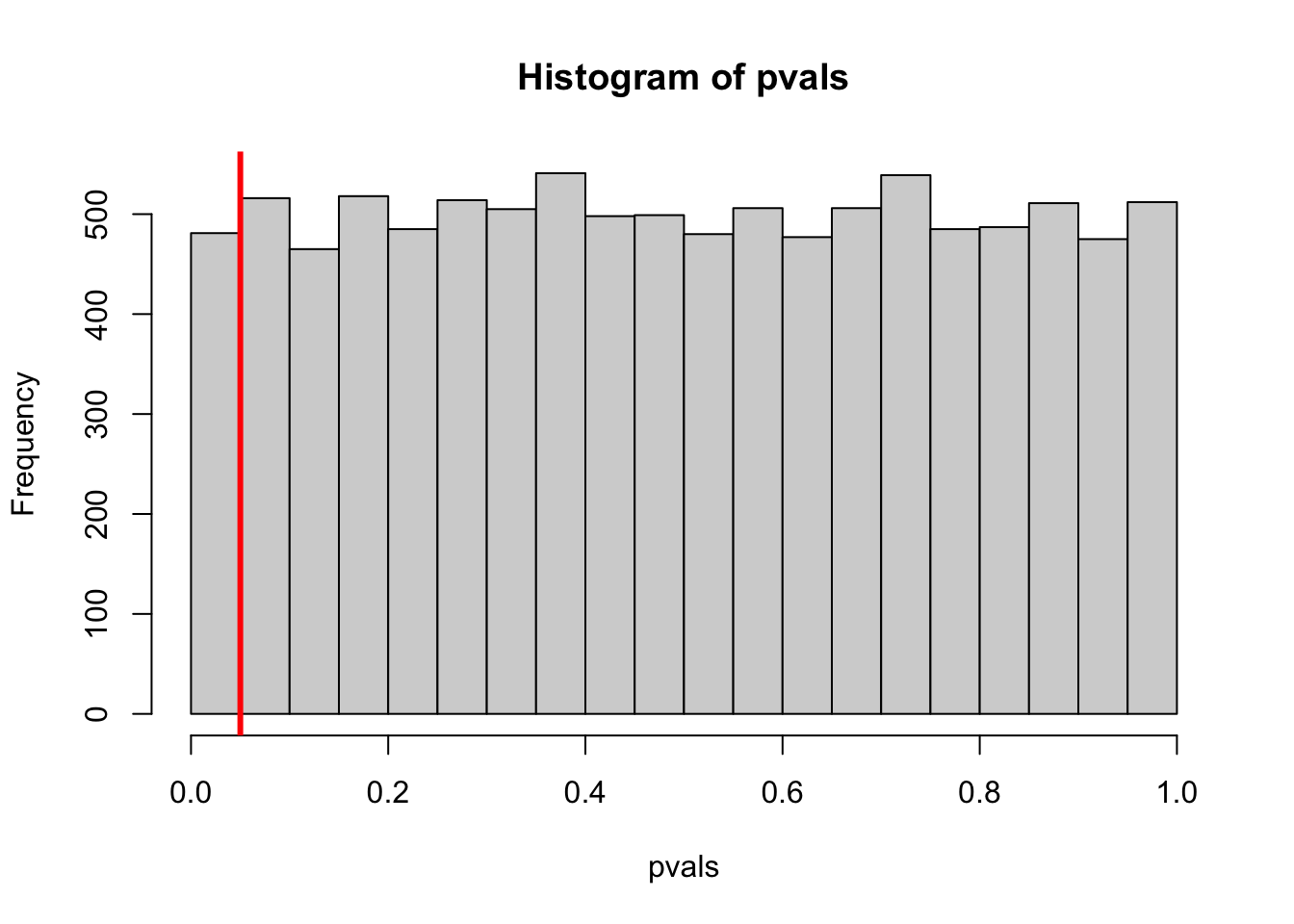
The histogram below shows all of the p-values we generated. The 5% cutoff isn’t anything special - a test at the 10% level will falsely reject the null 10% of the time. A test at the 90% level will falsely reject the null 90% of the time!
## Fun fact: under the null hyothesis, all p-values are equally likely## this fun fact is not relevant to this course.hist(pvals, breaks =seq(0, 1, 0.05))abline(v =0.05, col ="red", lwd =3)
The Probability of Type 2 Errors
For a two-sided test, our hypotheses are: \[\begin{align*}
H_0: \mu &= \mu_0\\
H_A: \mu &\ne \mu_0\\
\end{align*}\]
If the null is actually false3, what’s \(\mu\)? All we know is that it isn’t\(\mu_0\).4 It could be a little above \(\mu_0\), in which case it might be hard to reject \(\mu_0\). It could be a far above \(\mu_0\), in which case it might be easy to reject \(\mu_0\).
Easy to reject \(\mu_0\) since it’s so far from \(\mu\) (high power)
Hard to not reject the false \(\mu_0\) (low Type 2)
Power is our ability to correctly reject a false null hypothesis, and is defined as 1 - P(Type 2 Error)
Note that these examples are both missing the Standard Error, which incorporates sample size. The power depends on the distance between \(\mu\) and \(\mu_0\) relative to the standard error, not just the population standard deviation. We can partially control the standard error by having a better study design5 and a larger sample size, both of which would give us more power.
Power by Simulation (DIY)
The following code calculates the power. Run it many times, changing \(\mu_0\), \(\sigma\), and \(n\) to see what happens to the power.
## Set parametersmu <-0# don't change this, but change the other parametersmu_0 <-0.1sigma <-0.5n <-50## Record p-valsp_vals <-c()for(i in1:10000){ newsample <-rnorm(n, mu, sigma) p_vals[i] <-2* (1-pnorm(abs(mean(newsample)), 0, sigma/sqrt(n)))}## The proportion of times the null was (correctly) rejectedmean(p_vals <0.05) # Power
[1] 0.0483
mean(p_vals >0.05) # P(Type 2 Error)
[1] 0.9517
11.5 Multiple Comparisons
Suppose we have a coin that’s heads 5% of the time. What’s the probability of at least one heads in 10 flips?
As we saw in previous lectures: P(at least 1 heads in 10 flips) = 1 - P(no heads in 10 flips). We can calculate this in R:
1-dbinom(0, size =10, prob =0.05)
[1] 0.4012631
Why did I do go back to flipping coins? Did I forget which chapter I’m in?
Consider the following problem:
Suppose you’re testing 10 hypotheses at the 5% level. Assuming all of the null hypotheses are true, what’s the probability that at least one of them is significant?
Since we’re testing at the 5% level, P(Type 1 Error) = 0.05, so
P(\(\ge\) 1 rejection in 10 hypotheses) =
1-dbinom(0, size =10, prob =0.05)
[1] 0.4012631
In other words, there’s about a 40% chance that we’d get at least one significant result even though all of the null hypotheses are true.6
The Multiple Comparisons Problem
When checking more than one hypothesis, the probability of an error increases!
This happens for both Type 1 and Type 2 errors, but is especially important for Type 1 errors. If you test \(n\) errors at the \(\alpha\)% level, then the probability of a Type 1 error is \(1 -(1 - \alpha)^n\).
So how do we avoid the multiple comparisons problem? There are generally two ways to do it:
Set a Family-Wise Error Rate, rather than an error rate for individual hypothesis tests.
If you’re going to check 10 p-values, use a smaller cutoff.
There are several ways to do this, with the most popular being the Bonferroni correction: for m values, a cutoff of \(\alpha/m\) will result in rejecting at least one test \(\alpha\)% of the time. For example, if you want a test at the 5% level but you’re testing 10 values, you should reject any individual hypothesis only if the p-value is less than \(\alpha/m = 0.05/10\).
Only check one p-value!
For most studies, you should have single, well-defined hypothesis. State this hypothesis ahead of time, do all of your data preparation and get it loaded into R, then only test that hypothesis.
If you check a second hypothesis, then your significance level is a lie! Testing two true null hypotheses at the 5% level will result in a significant result 9.75% of the time.
Failure to account for multiple hypothesis testing is bad science and it’s a path to the dark side. Consider this fantastic tool by fivethirtyeight. Play around with it - by checking a bunch of hypotheses, you can hack your way into finding one that supports your own point of view! In this particular example, your goal is to prove that either (a) the economy does better when a democrat in the white house or (b) the economy does better when a republican is in the white house. Both of these can be demonstrated with a statistically significant result if you check enough hypotheses!
Let’s return to the 👽 aliens example. We observed an abberation that only happens in 0.0001% of the pictures taken. However, we took thousands of pictures! Even though this event is rare, it had many chances to happen. This is exactly what multiple hypothesis testing is demonstrating: rare events will happen if you give them enough chances! Rejecting the null when it is actually true is a rare event, but it can easily happen if we check a lot of p-values!
11.6 Summary
Type 1 Error: Reject a true null
Probability is \(\alpha\)
Type 2 Error: Fail to reject a false null
Probability depends on the distance between \(\mu\) and \(\mu_0\), relative to the standard error. In more advanced classes, you will calculate this or have something to calculate it for you.
Multiple comparisons problem: The more hypotheses you test, the more likely it is that at least one of them is falsely labelled significant.
To prevent this, stop checking so many p-values or adjust your expectations!
11.7 Self-Study Questions
We set up the null hypotheses as “nothing interesting is going on”. In light of this, explain why power is a good thing.
If we’re testing 5 hypotheses, what significance level should we use for each such that P(at least one type 1 error) = 0.05?
If we have the hypotheses \(H_0:\mu = 1\) versus \(H_0:\mu = 2\), we can directly calculate the power. Run the following code to open the Shiny app, and interpret the results.
p-values are the probability of observing our data by chance alone.
True
False
Q2
p-values are the probability of getting data at least this extreme under the null hypothesis.
True
False
Q3
p-values are a measure of evidence against the null hypothesis.
True
False
Q4
\(H_0\) is TRUE
\(H_0\) is FALSE
Don’t Reject
Good!
Type 2 Error
Reject
Type 1 Error
Hooray!
In a particular hypothesis test, rejecting the null means diagnosing a patient with cancer.
Select all that are true.
A low significance level means that I require strong evidence before I declare cancer.
A high power means that I’m more likely to diagnose someone with cancer, assuming they actually have cancer.
Low type 2 error means that I am less likely to miss true cancer diagnoses.
The probability of type 1 error is equal to the significance level \(\alpha\).
Q5
\(H_0\) is TRUE
\(H_0\) is FALSE
Don’t Reject
Good!
Type 2 Error
Reject
Type 1 Error
Hooray!
In a particular hypothesis test, rejecting the null means diagnosing a patient with cancer.
Which of the following is true about Type 1 and Type 2 error?
Increasing \(\alpha\) means I’m less likely to diagnose someone with cancer.
High power means I’m more likely to diagnose someone with cancer who actually has cancer.
The probability that my diagnosis is correct is 1 - P(Type 2 error).
A smaller significance level means I’ll have less power.
11.9 Crowdsourced Questions
The following questions are added from the Winter 2024 section of ST231 at Wilfrid Laurier University. The students submitted questions for bonus marks, and I have included them here (with permission, and possibly minor modifications).
A type 1 error occurs when?
A null hypothesis is not rejected but should be rejected
A null hypothesis is rejected but should not be rejected
A test statistic is incorrect
None of the above are correct
Solution
is the correct answer – In statistical hypothesis testing, a type 1 error (also known as a “false positive”) refers to the situation where the null hypothesis is incorrectly rejected when it is actually true. This means that the test concludes there is a significant effect or difference when, in reality, there is none.
Bottles of water have a label stating that the volume is 14 oz. A ST231 class suspects the bottles are under‐filled and plans to conduct a test. A Type I error in this situation would mean:
The ST231 class concludes the bottle has less than 14 oz, when the mean actually is 14 oz
The ST231 class concludes the bottles has less than 14 oz when the mean actually is less than 14 oz
The ST231 class has evidence that the label is incorrect
A type 1 error does not occur but a Type 2 error does
Solution
is the correct answer because it aligns with the definition of a Type I error, which occurs when the null hypothesis (in this case, that the bottles have 14 oz) is incorrectly rejected, leading to the conclusion that the bottles have less than 14 oz when, in fact, they do have 14 oz.
A researcher conducts a hypothesis test with a significance level of 0.05. What does this significance level represent?
There is a 5% chance of making a Type l error.
There is a 5% chance of making a Type ll error.
There is a 95% confidence level in the results
There is a 95% chance of the null hypothesis being true.
Solution
a is the correct answer - the significance level 0.05 meant that there is a 5% chance of committing a Type l error, which means to reject the null hypothesis when it is actually true. The significance level is usually chosen by researchers to control the risk of making a Type l error, it does not directly represent the probability of Type ll error. The significance level does not specifically represent the confidence interval.
A researcher is designing a study to determine the effectiveness of a new drug in reducing blood pressure. They want to make sure that their study has enough power to detect a clinically meaningful difference in blood pressure if it actually exists. Which of the following actions would increase the statistical power of the study.
Increasing the sample size
Decreasing the significance level
Lowering the effect size
Using a one-tailed test instead of a two-tailed test
Solution
a is the correct answer - increasing the sample size would increase the statistical power. A larger sample size gives more information and reduces the variability in the estimate of the population parameter (mean or the effect size), making it more precise and easier to detect smaller effects. The rest of the options don’t increase the statistical power.
A new production procedure, according to the corporation, lowers the average product fault rate to less than 1%. To assess this assertion, a statistical test is performed. A defect rate of less than 1% is suggested by the alternative hypothesis (H1), contrary to the null hypothesis (H0), which maintains that the defect rate stays at 1% or higher. The business rejects the null hypothesis after determining that the new manufacturing procedure effectively lowers the defect rate based on its analysis of the data. In this case, what kind of mistake might the corporation have made?
The company correctly rejected the null hypothesis when the defect rate remains at 1% or higher.
The company erroneously rejected the null hypothesis when the defect rate remains at 1% or higher.
The company correctly failed to reject the null hypothesis when the defect rate is less than 1%.
The company erroneously failed to reject the null hypothesis when the defect rate is less than 1%.
Solution
The right answer is option (b). In this instance, the corporation made a Type 1 error by mistakenly rejecting the null hypothesis (H0) when it was true (the failure rate is still 1% or greater). Due to a Type 1 error, the business came to the false conclusion that the new manufacturing method effectively lowers the failure rate, which could have led to poor resource allocation and decision-making.
A team of experts is looking into how a new teaching strategy affects maths students’ performance. In order to identify any significant changes in test results between the old and new teaching approaches, they want to make sure that their study has enough statistical power. Which of the following steps would most effectively boost their study’s statistical power?
Increasing the sample size of students participating in the study.
Decreasing the alpha level (significance level) used for hypothesis testing.
Reducing the effect size of the difference in test scores between the teaching methods.
Changing from a two-tailed test to a one-tailed test.
Solution
A is the right answer. The study’s statistical power would be improved by expanding its sample size. More information is available and the estimate of the population parameter’s variability is decreased with a larger sample size, which facilitates the detection of minor impacts. There would be no direct increase in statistical power with options B, C, and D. While it wouldn’t impact statistical power, lowering the alpha threshold would lessen the possibility of Type I mistakes. Reducing the effect size would make it more difficult to identify differences, and switching from a two-tailed test to a one-tailed test would not automatically result in a higher power.
A researcher is conducting a study to evaluate the effectiveness of a new diagnostic test for a rare disease. The null hypothesis is that the diagnostic test correctly identifies individuals without the disease, while the alternative hypothesis is that the test incorrectly identifies individuals without the disease as positive. The significance level is set at 0.05.
Describe Type I and Type II errors in the context of this study.
What are the consequences of making each type of error?
How would you reduce the risk of each type of error in this study?
Solution
Type I Error occurs when the researcher incorrectly rejects the null hypothesis, deciding that the diagnostic test shows the individuals without the disease as positive when, in fact, they do not have the disease. Type II Error occurs when the researcher fails to reject the null hypothesis, concluding that the diagnostic test correctly identifies individuals without the disease when, in reality, they have the disease.
The consequences of Type I Error results in unnecessary medical interventions, psychological distress for individuals incorrectly diagnosed as positive, and increased healthcare costs. Type II Error, on the other hand, may result in missed diagnoses, delayed treatment, progression of the disease, and potential harm to patients due to lack of appropriate medical care.
To reduce the risk of Type I Error, the researcher can ensure careful validation of the diagnostic test through extensive testing on control groups and ensuring proper calibration to minimize false positives. Additionally, rigorous statistical analysis and replication of results can help verify the test’s accuracy. To minimize the risk of Type II Error, the researcher can increase the sample size to improve statistical power, as a result reducing the likelihood of missing true positives. The researcher can also conduct thorough follow-up examinations or use diagnostic methods to confirm or rule out diagnosis made by the test.
A study is being conducted to evaluate the effectiveness of a new treatment method in treating a specific medical condition. The researcher is considering the sample size for the study. Which of the following statements best describes the relationship between sample size and statistical power in this scenario?
Increasing the sample size may or may not affect statistical power depending on the effect size.
Increasing the sample size will always increase statistical power.
There is an inverse relationship between sample size and statistical power.
Increasing the sample size generally increases statistical power, but other factors such as effect size may also play a role.
Solution
Increasing the sample size generally increases statistical power, but other factors such as effect size may also play a role. As the sample size increases, so does the power of the significance test. This is because a larger sample size restricts the distribution of the test statistic, meaning that the standard error of the distribution is reduced and the acceptance region is reduced which as a result increases the level of power.
We can think long and hard about it before seeing the data, but once we see the data we are commited to a particular significance level. Anything else is borderline fraud, depending on the circumstances.↩︎
Recall: the p-value is the probability of a result that is at least as extreme assuming that the null hypothesis is true!↩︎
False in the population, not just rejected due to a sample.↩︎
I once saw a bag in a grocery store with a label that said “It’s Not Bacon”. I had no idea what was in that bag. In the video I said it was kale, but that turns out to be false.↩︎