\[\begin{align*}
\underline\epsilon^T\underline\epsilon &= (Y - X\underline\beta)^T(Y - X\underline\beta)\\
&= ... = Y^TY - 2\underline\beta^TX^TY + \underline\beta^TX^TX\underline\beta
\end{align*}\] We then take the derivative with respect to \(\underline\beta\). Note that \(X^TX\) is symmetric and \(Y^TX\underline\beta\) is a scalar.. \[\begin{align*}
\frac{\partial}{\partial\underline\beta}\underline\epsilon^T\underline\epsilon &= 0 - 2X^TY + 2X^TX\underline\beta
\end{align*}\]
For the 1 predictor case, verify that the equations look the same!
Setting to 0, rearranging, and plugging in our data gets us the Normal equations: \[\begin{align*}
X^TX\underline{\hat\beta} &= X^T\underline y
\end{align*}\]
Facts
The solution to the normal equations satisfies: \[X^TX\underline{\hat\beta} = X^T\underline y\]
No distributional assumptions.
If \(X^TX\) is invertible, \(\hat{\underline\beta} = (X^TX)^{-1}X^T\underline y\).
\(\hat{\underline\beta}\) is a linear transformation of \(\underline y\)!
This is the same as the MLE.
\(E(\hat{\underline\beta}) = \underline\beta\) and \(V(\hat{\underline\beta}) = \sigma^2(X^TX)^{-1}\).
This is the smallest variance amongst all unbiased estimators of \(\underline\beta\).
Example Proof Problems
Prove that \(\sum_{i=1}^n\hat\epsilon_i\hat y_i = 0\).
Prove that \(\sum_{i=1}^n\hat\epsilon_i = 0\).
Prove that \(X^TX\) is symmetric. Is \(A^TA\) symmetric in general?
Show the code
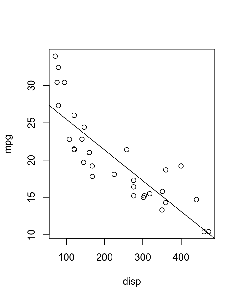
## Demonstration that they're true (up to a rounding error)mylm <-lm(mpg ~ disp, data = mtcars)sum(resid(mylm) *predict(mylm))
[1] -2.664535e-14
Show the code
mean(resid(mylm))
[1] -1.12757e-16
Show the code
X <-model.matrix(mpg ~ disp, data = mtcars)all.equal(t(X) %*% X, t(t(X) %*% X))
[1] TRUE
Analysis of Variance (Corrected)
Source
\(df\)
\(SS\)
Regression (corrected)
\(p - 1\)
\(\underline{\hat{\beta}}^TX^T\underline y - n\bar{y}^2\)
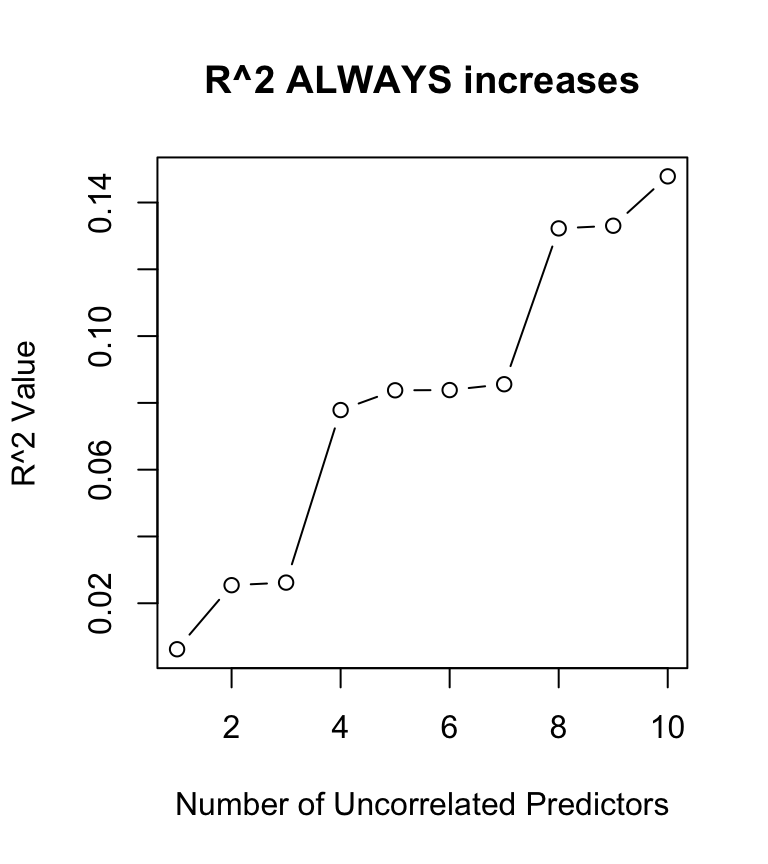
nx <-10# Number of uncorrelated predictoresuncorr <-matrix(rnorm(50*(nx +1)), nrow =50, ncol = nx +1)## First column is y, rest are xcolnames(uncorr) <-c("y", paste0("x", 1:nx))uncorr <-as.data.frame(uncorr)rsquares <-NAfor (i in2:(nx +1)) { rsquares <-c(rsquares,summary(lm(y ~ ., data = uncorr[,1:i]))$r.squared)}plot(1:10, rsquares[-1], type ="b",xlab ="Number of Uncorrelated Predictors",ylab ="R^2 Value",main ="R^2 ALWAYS increases")
Works (poorly) for comparing different models on different data.
In general you should use \(R^2_a\), but always be careful.
5.2 Prediction and Confidence Intervals (Again)
\(R^2\) and \(F\)
Recall that \[
F = \frac{MS(Reg|\hat\beta_0)}{MSE} = \frac{SS(Reg|\hat\beta_0)/(p-1)}{SSE/(n-p)} \sim F_{p-1, n-p}
\]
From the definition of \(R^2\), \[\begin{align*}
R^2 &= \frac{SS(Reg|\hat\beta_0)}{SST}\\
&= \frac{SS(Reg|\hat\beta_0)}{SS(Reg|\hat\beta_0) + SSE}\\
&= \frac{(p-1)F}{(p-1)F + (n-p)}
\end{align*}\] Conclusion: Hypothesis tests/CIs for \(R^2\) aren’t useful. Just use \(F\)!
Correlation of \(\hat\beta_0\), \(\hat\beta_1\), \(\hat\beta_2\), etc.
With a different sample, we would have gotten slightly different numbers!
If the slope changed, the intercept must change to fit the data
(and )
The parameter estimates are correlated!
Similar things happen with multiple predictors!
This correlation can be a problem for confidence regions
In simple linear regression, \[
(X^TX)^{-1} = \frac{1}{nS_{XX}}\begin{bmatrix}\sum x_i^2 & -n\bar x\\-n \bar x & n\end{bmatrix}
\]
so the correlation is 0 when \(\bar x = 0\)!
It’s common practice to mean-center the predictors for this very reason!
For 2 or more predictors, \((X^TX)^{-1}\) has a more complicated expression.
The correlation of the \(\beta_j\)s is a function of the correlations in the data.
Prediction and Confidence Intervals for \(Y\)
\(\hat Y = X\hat\beta\).
A confidence interval around \(\hat Y\) is based on the variance of \(\hat\beta\).
\(\hat Y \pm t * se(X\hat\beta)\)
\(Y_{n+1} = X\beta + \epsilon_{n+1}\)
A prediction interval around \(Y_{n+1}\) is based on the variance of \(\hat\beta\)and\(\epsilon\)!
\(\hat Y_{n+1} \pm t * se(X\hat\beta + \epsilon_{n+1})\)
5.3 Exercises
Prove that \(\sum_{i=1}^n\hat\epsilon_i\hat y_i = 0\).
Prove that \(\sum_{i=1}^n\hat\epsilon_i = 0\).
Prove that \(X^TX\) is symmetric. Is \(A^TA\) symmetric in general?
Simulate data with \(n = 50\), \(p = 11\), and \(\beta_1 = \beta_2 = ... = \beta_10 = 0\). Check the individual t-tests for whether the slopes are 0, and the overall F-test. Do this multiple times. Do you find a significant result from one of the t-tests but not the overall F-test? What about vice-versa?
Solution
n <-50p <-11X <-matrix(data =c(rep(1, n),runif(n * (p -1), -5, 5)),ncol = p)beta <-c(p -1, rep(0, p -1)) # beta_0 = 10, will not affect resultsy <- X %*% beta +rnorm(n, 0, 3)mydf <-data.frame(y, X[, -1])mylm <-lm(y ~ ., data = mydf)summary(mylm)
In my run (this will be different each time you run it), one of the slopes was found to be significant! This is a Type 1 error - we found a significant result where we shouldn’t have.
However, the F-test successfully found that the overall fit is not significantly better than a model without any predictors. F-tests exists to prevent Type 1 errors!
As a side note, check out the difference between the Multiple R-squared and Adjusted R-squared. Which one would you believe in this situation?
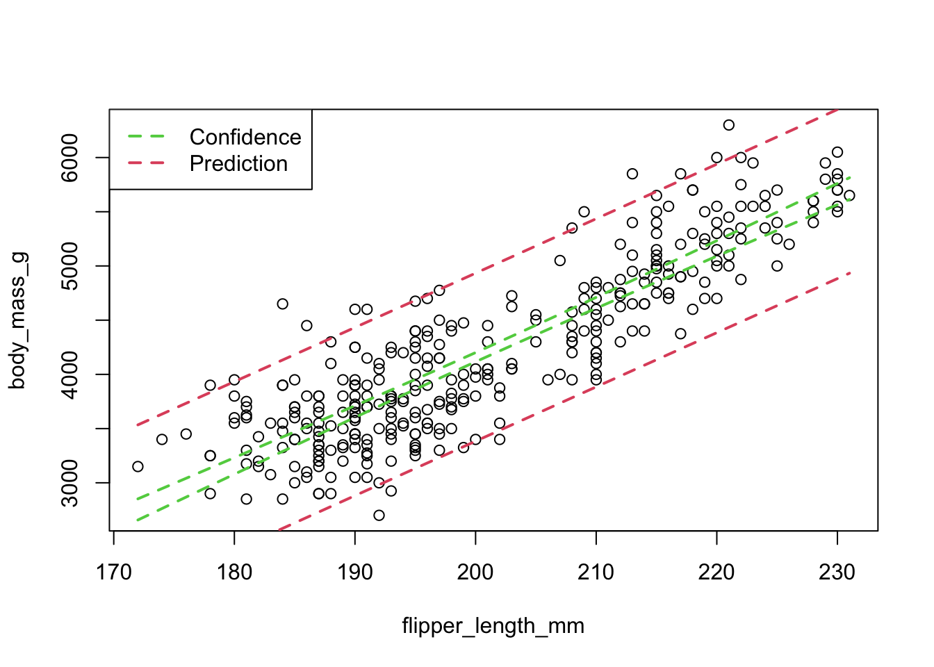
Plot the confidence intervals and the prediction intervals for a simple linear regression of body mass versus flipper length for penguins. Do this for a lot of points, and interpret the difference between the two.
library(palmerpenguins)penguins <- penguins[complete.cases(penguins),]peng_lm <-lm(body_mass_g ~ flipper_length_mm, data = penguins)
Solution
library(palmerpenguins)penguins <- penguins[complete.cases(penguins),]peng_lm <-lm(body_mass_g ~ flipper_length_mm, data = penguins)# confidence intervals along all flipper lengthsflippers <-seq(from =min(penguins$flipper_length_mm),to =max(penguins$flipper_length_mm), length.out =100)confi <-predict(peng_lm, newdata =data.frame(flipper_length_mm = flippers), interval ="confidence")predi <-predict(peng_lm, newdata =data.frame(flipper_length_mm = flippers), interval ="prediction")plot(body_mass_g ~ flipper_length_mm, data = penguins)lines(x = flippers, y = confi[, "upr"], col =3, lwd =2, lty =2)lines(x = flippers, y = confi[, "lwr"], col =3, lwd =2, lty =2)lines(x = flippers, y = predi[, "upr"], col =2, lwd =2, lty =2)lines(x = flippers, y = predi[, "lwr"], col =2, lwd =2, lty =2)legend("topleft", legend =c("Confidence", "Prediction"), col =3:2, lwd =2, lty =2)
The confidence “band” is much thinner than the prediction band! With this many points, the model is pretty sure about the slope and intercept (i.e. \(\hat y_i\)); a new sample would be expected to produce a similar line.
However, even though the model knows about the slope and intercept of the line, there’s still lots of uncertainty around an unobserved point \(\hat y_{n + 1}\).
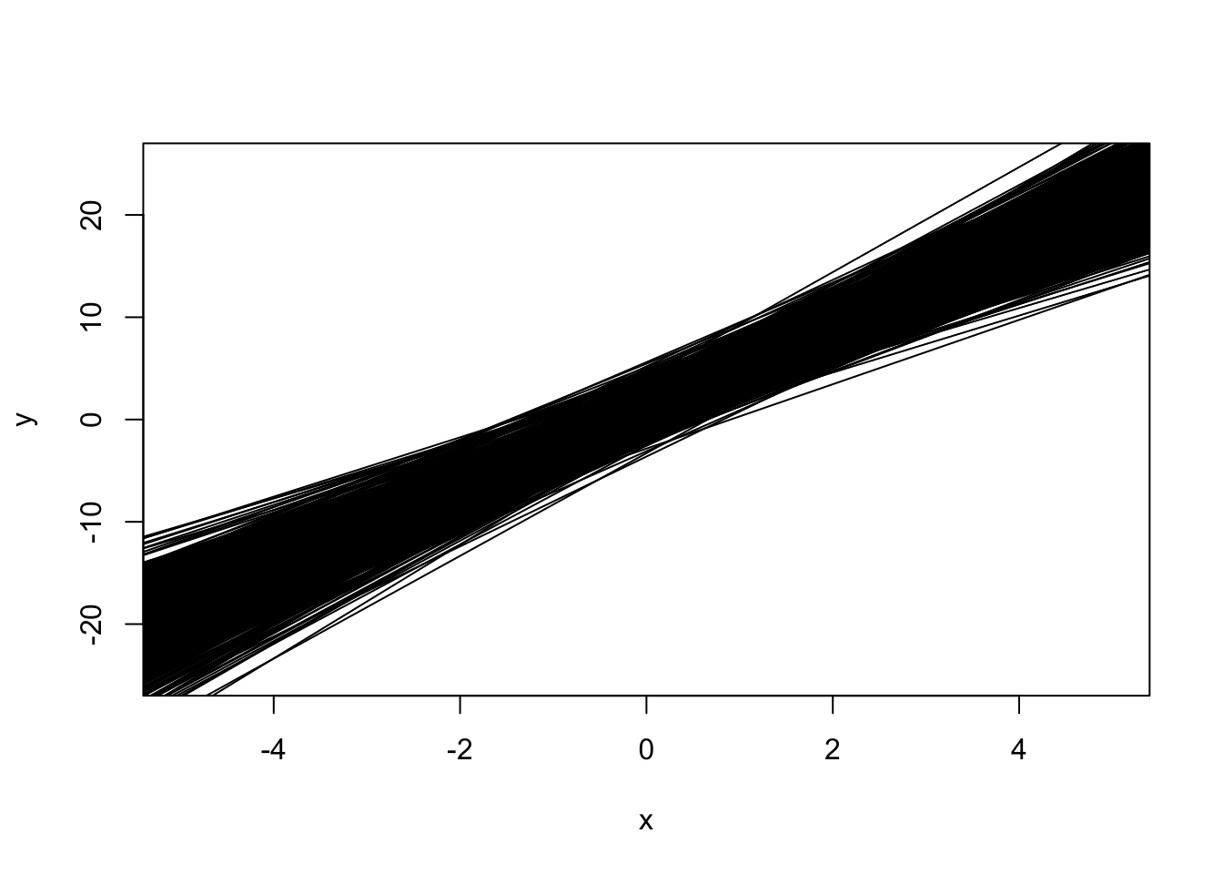
Use a simulation to demonstrate a confidence interval for \(\hat y_i\) (an observed data point). For a model \(y_i = 1 + 4x_i + \epsilon_i\), \(\epsilon_i \sim N(0, 16)\), \(n = 30\), simulate 100 data sets, calculate the line, and add it to a plot. What do you notice about the shape? Why is this?
Solution
n <-30x <-runif(n, -5, 5)plot(NA, xlim =c(-5, 5), ylim =c(-25, 25), xlab ="x", ylab ="y")for (i in1:1000) { y <-1+4* x +rnorm(n, 0, 8)abline(lm(y ~ x))}
It looks kind of like a bowtie!
As mentioned in lecture, the model can be seen as fitting a point at \((\bar x, \bar y)\), then finding a slope that fits the data well. If we got the exact same value for \(\bar y\) every time, every single line would converge at the point \((\bar x, \bar y)\)!
We also saw that the variance of \(\hat y_i\) is minimized at \(\bar x\), and this plot demonstrates this.