13 Transformations
13.1 Transformations
Transforming the Predictors
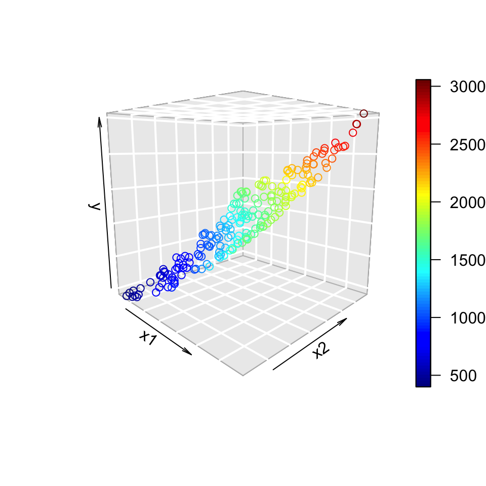
Suppose we found that the following second order polynomial model was a “good” fit: \[ y_i = \beta_0 + \beta_1x_{i1} + \beta_{11}x_{i1}^2 +\beta_2x_{i2} + \beta_{22}x_{i2}^2 + \beta_{12}x_{i1}x_{i2} + \epsilon_i \]
Now consider the model: \[ \ln(y_i) = \beta_0 + \beta_1x_{i1} + \beta_2x_{i2} + \epsilon_i \]
- 3 parameters instead of 6!
- No interaction term!
- If we’re okay with the log scale for \(y\), it’s easier to interpret.
Transforming the predictors
Original scale
Log scale
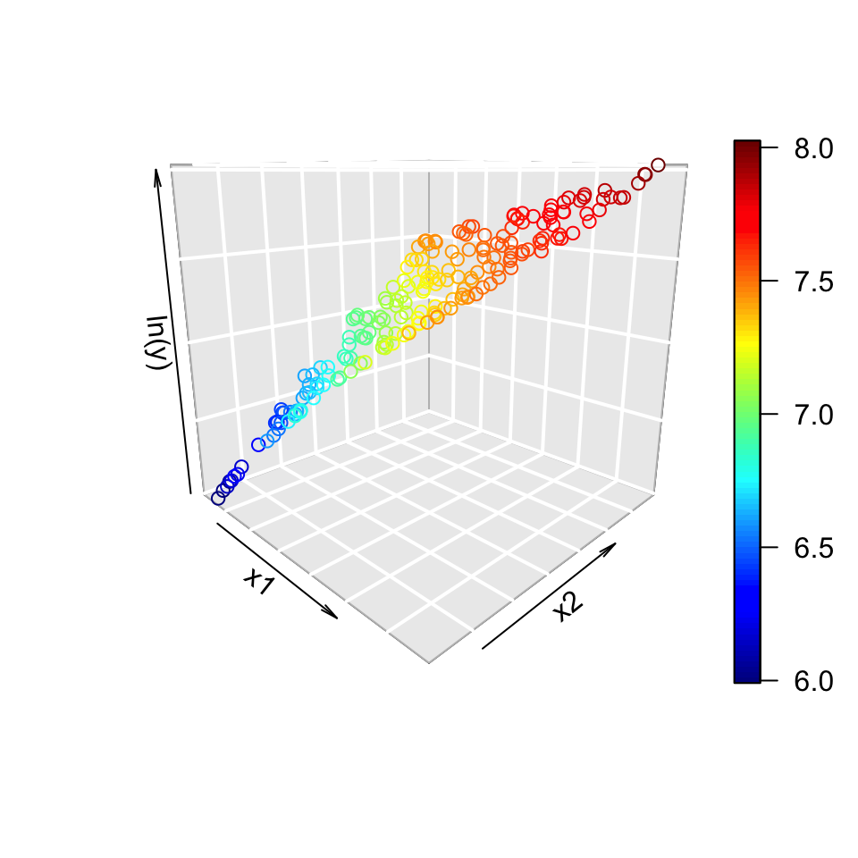
The logarithm made it simpler, even if it’s still not quite right.
The code below can be run on your local machine (the rgl library needs to make it’s own window, which it can’t do in any online format).
Play around with some transformations of \(x_1\) and \(x_2\), then play around with transformations of \(y\)!
library(rgl)
set.seed(2112)
n <- 200
x1 <- runif(n, 3, 10)
x2 <- runif(n, 3, 10)
y <- 20 + 5*x1 + 15*x1^2 + 5*x2 + 15*x2^2  + 2*x1*x2 + rnorm(n, 0, 2)

rgl::plot3d(x1, x2, y)
Consequences of Logarithms
Consider the simple model \(E(y_i) = \beta x^2\). Taking the logarithm of both sides: \[ \ln(E(y_i)) = \ln(\beta) + 2\ln(x) := \beta_0 + \beta_1 \ln(x) \] and we have something that looks more like a linear model.
- Note that, instead of \(x^2\), \(x^{2.1}\) would also work as a model.
- The power of \(x\) is estimated.
- It’s also possible that the log scale is the correct scale for \(y\)
- \(E(\ln(y_i)) = \beta_0 + \beta_1x\)
- In other words, don’t get too bogged down by whether we take the ln of \(x\).
Logarithms and Errors
If we believe that the log scale is a better scale for \(y\), we may postulate the model: \[ \ln(y_i) = \beta_0 + \beta_1\ln x_{i1} + \beta_2\ln x_{i2} + \epsilon \] which implies that the orginal scale for \(y\) has the form: \[ y_i = e^{\beta_0}x_{i1}^{\beta_1}x_{i2}^{\beta_2}e^{\epsilon_i} \] The errors are multiplicative!!!
- Option 1: Accept this
- Allows us to use least squares.
- Option 2: Use the model \(y_i = e^{\beta_0}x_{i1}^{\beta_1}x_{i2}^{\beta_2} + \epsilon_i\)
- Might be better, but requires a bespoke estimation algorithm.
Are we also taking the log of \(x\)?
No (the usual case)
\[ \ln(E(y_i)) = \beta_0 + \beta_1x_{i1} + \beta_2 x_{i2} \]
\[ \implies y_i = e^{\beta_1}e^{\beta_1x_{i1}}e^{\beta_2x_{i2}}e^{\epsilon_i} \]
- Usually used in order to make the plot look more linear.
Yes (if there’s good reason)
\[ \ln(E(y_i)) = \beta_0 + \beta_1\ln x_{i1} + \beta_2 \ln x_{i2} \]
\[ \implies y_i = e^{\beta_1}x_{i1}^{\beta_1}x_{i2}^{\beta_2}e^{\epsilon_i} \]
- Usually used if we think the form \(y = \beta_0x^\beta e^\epsilon\) is the correct form.
Secret third option: transform the \(x\) values only (example: polynomial regression).
You may notice that the first row in each column transforms \(E(y_i)\), but the second is the transform of \(y_i\). This is not a mistake. We transform the expected relationship between \(X\) and \(y\), then fit the model assuming that the residuals are additive so we can use our usual least squares estimators. To transform them back, we don’t know the residuals and therefore they get caught up in the transformation.
General Practice
We often simply use the model \(\ln \underline y = X\beta + \underline \epsilon\) and do everything on the log scale.
- Simpler, but still useful.
- Good predictions of \(\ln y_i\) can be transformed to good predictions of \(y_i\).
- If there’s a good reason to transform the \(x\) values, we’ll try that first.
- E.g. stopping distance \(\propto\) speed\(^2\); decibels are on the log scale but we might want them on the raw sale, etc.
In general: Decide on a functional relationship between \(f(y)\) and \(X\), then use additive errors on the scale of \(f(y)\).
This has consequences for the residuals.
13.2 Residuals in Transformed Space
Variance Stabilization
The two main purposes of transformations:
- Fit non-linear functional forms.
- Stabilize the variance!
- Scale-Location plot in the R defaults.
For example, the log function brings large values down a lot, small values down a little.
- The scale of large residuals is decreased more than the scale of small residuals.
\(f(\underline y) = X\beta + \underline\epsilon\)
The estimated residuals are \(\hat\epsilon_i = f(y_i) - \widehat{f(y_i)}\)
- Note the awkwardly long hat!
- We’re estimating the value of the function, not the value of \(y_i\).
- If \(f(y_i) - \widehat{f(y_i)} = f(y_i - \widehat{y_i})\), then the original function must have been linear (and a transformation was useless).
- We’re assuming \(\epsilon_i\stackrel{iid}{\sim} N(0, \sigma^2)\), which is difficult to translate to \(f^{-1}(X\beta + \underline\epsilon)\).
- In the special case of \(\ln\), \(\exp{\epsilon_i} \sim \text{LogNormal}(0, \sigma^2)\).
- No assumption of independence on the original scale!!!
- We assume that the residuals have the same variance on the transformed scale.
- Likely not true for the original scale of \(y\).
Some Good News
If \((a,b)\) is a \((1-\alpha)\) CI on the scale of \(f(y)\), then \((f^{-1}(a), f^{-1}(b))\) is a valid CI on the scale of \(y\).
- It’s not the only valid CI!
- Note that it’s not a symmetric CI!
- Works for \(y\) as well as the \(\beta\) parameters.
- Transformation might induce dependence among the parameters.
- A CI for \(\beta_1\) is useless if there’s high covariance with \(\beta_2\).
Example: Dugongs
Check the diagnostic plots for the following models!
This is that in-browser R magic that we’ve seen before! Also ask yourself what it means for the log of age to increase with the length of the dugong. Is the log easy to interpret? Do the x and y variables make sense like this?
13.3 Choosing Transformations
Methods for Choosing Transformations
- Theory.
- If theory says that the log transform makes sense, use that.
- Don’t even consider the next steps. Just go with theory.
- Example: Forest fire burn sizes are right skewed, the log-transform makes sense.
- If theory says that the log transform makes sense, use that.
- Experimentation after looking at the Scale-Location plot.
- If log or sqrt don’t work, move on to step three.
- The Box-Cox Transformation
- Finds an appropriate transformation using maximum likelihood.
Box-Cox
We use the transformation: \[ V = \begin{cases} \frac{Y^\lambda - 1}{\lambda \dot{Y}^{\lambda - 1}} & \text{if }\lambda \ne 0\\ \dot{Y}\ln(Y) & \text{if }\lambda = 0 \end{cases} \] where \(\dot Y\) is the geometric mean of \(y\).
\(\lambda\) is chosen through maximum likelihood
- Essentially, refit with each value of \(\lambda\) and see which minimizes the residual variance.
- Plot the likelihhods and choose the highest.
Simpler Box-Cox
The textbook recommends the previous formula, however R uses: \[ W = \begin{cases} \frac{Y^\lambda - 1}{\lambda} & \text{if }\lambda \ne 0\\ \ln(Y) & \text{if }\lambda = 0 \end{cases} \]
Notice:
- \(\lambda \approx -1 \implies\) inverse transformation.
- \(\lambda \approx 0 \implies\) log transformation.
- \(\lambda \approx 0.5 \implies\) sqrt transformation.
- \(\lambda \approx 1 \implies\) no transformation.
- \(\lambda \approx k, k\in\mathbb{Z} \implies\) use \(y^k\).
- There’s no \(\lambda\) for \(exp(y)\)!
Variance of \(\lambda\)
If we had a different data set, we’d get a different value of \(\lambda\)!
R reports the the log-likelihood values, along with the top 5%.
- Anything in the top 5% is reasonable.
- It’s not an exact science.
- Usually, we check the best \(\lambda\) values and round to something nice.
- log, sqrt, squared, inverse, etc.
Example
- Generate
y ~ log(x), try fittingy ~ log(x)and also a transformation fory. - Generate
log(y) ~ x, try fittingy ~ exp(x)and alsolog(y) ~ x. - Generate
log(y) ~ log(x), try various transformations ofyandx. - Generate
y ~ x^2, try various transformations ofyandx. - Generate
y^2 ~ x, try various transformations ofyandx.
After some exploring, you should find that the log and sqrt transformations cover most situations adequately. Fitting the correct model is obviously best, but we can never know what the correct model is!!!
As practice, try writing out all models in the form \(y = g(f(x) + \epsilon)\) to see how the error terms get affected. For example, generating data like \(log(y) = log(x) + epsilon\) implies the model \(y = exp(log(x) + \epsilon)\), which does not simplify due to the additive error term in the exponential.
Summary
- Choosing a transformation:
- Theory
- Exploration
- Rounded value from Box-Cox.
- Working with a transformation:
- Choose functional form, assume additive errors (usually, not always!)
- Stay on the transformed scale
- All assumptions about residuals apply to the transformed scale!
To be useful, all transformations should consider the context of the problem!