16 Dummy Variables
16.1 0/1 Predictors
Dummy Coding
“Dummy” variables are just predictors that only take the values 0 and 1.
- 0 pairs of glasses versus 1 pair of glasses
- This is a count that can only be 0 or 1
- 0 means automatic, 1 means manual
- Arbitrary choice of 0/1
- 0 means off, 1 means on
- Natural choice of 0/1, but still arbitrary
Slopes with a Dummy Variable
Usual interpretation: as \(x\) increases by 1, \(y\) increases by \(\beta\).
This doesn’t go away, but we get a new interpretation!
- \(x\) can only increase by one (from 0 to 1).
- \(\beta\) is the difference in groups.
Note that we assume constant variance; this means the variance is the same in both groups
- Exact same assumptions as a t-test.
- (Different from a “Welch” t-test)
Categorical Variables
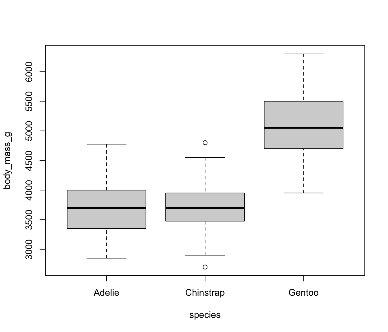
Consider the species column in penguins. We could code three dummy variables:
- \(I(species == Adelie)\)
- \(I(species == Chinstrap)\)
- \(I(species == Gentoo)\)
For brevity, \(I(Adelie)\) is the same as \(I(species == Adelie)\).
This would lead to the model: \[ y = \beta_0 + \beta_1I(Adelie) + \beta_2I(Chinstrap) + \beta_3I(Gentoo) \]
What’s the interpretation of the intercept here?
Categorical Variable Dummy Coding
Better: set one as a reference variable and let the intercept “absorb” it:
- \(I(species == Chinstrap)\)
- \(I(species == Gentoo)\)
This would lead to the model: \[ y = \beta_0 + \beta_1I(Chinstrap) + \beta_2I(Gentoo) \] where
- \(\beta_0\) is the mean of body mass for Adelie penguins.
- \(\beta_1\) is the difference in mean body mass between Adelie and Chinstrap.
- \(\beta_2\) is the difference in mean body mass for Adelie versus Gentoo.
- Difference between Chinstrap and Gentoo can be found with some cleverness.
Models with Categorical Variables
The model \(y = \beta_0 + \beta_1I(species == Chinstrap) + \beta_2I(species == Gentoo)\) is equivalent to: \[ y_i = \begin{cases}\beta_0 + 0 & \text{if }\; species == Adelie\\ \beta_0 + \beta_1 & \text{if }\; species == Chinstrap\\\beta_0 + \beta_2 & \text{if }\; species == Gentoo\end{cases} \]
This is equivalent to fitting an intercept-only model \(y = \beta_0\) for subsets of the data.
By putting them in the same model, we can easily test for significance.
The following code demonstrates that this is true - make sure you understand where each value is coming from!
Testing Significance
Show the code
summary(lm(body_mass_g ~ species, data = penguins))$coef Estimate Std. Error t value Pr(>|t|)
(Intercept) 3706.16438 38.13563 97.1837676 6.880362e-245
speciesChinstrap 26.92385 67.65243 0.3979732 6.909073e-01
speciesGentoo 1386.27259 56.90893 24.3594924 1.009947e-75So… is species significant?
Show the code
anova(lm(body_mass_g ~ species, data = penguins))Analysis of Variance Table
Response: body_mass_g
Df Sum Sq Mean Sq F value Pr(>F)
species 2 145190219 72595110 341.89 < 2.2e-16 ***
Residuals 330 70069447 212332
---
Signif. codes: 0 '***' 0.001 '**' 0.01 '*' 0.05 '.' 0.1 ' ' 1It’s an ESS test!!!
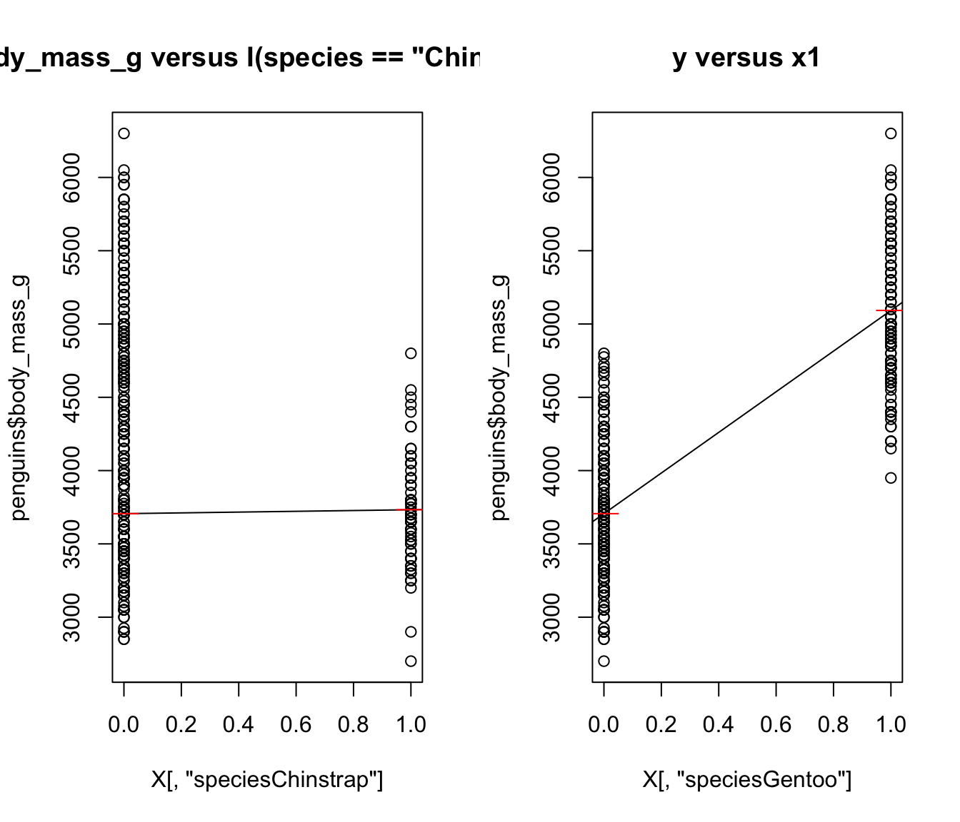
Plotting the Results (Correct, but Don’t Use This)
We fit a model with two predictors: \[ I(species == Chinstrap)\text{ and }I(species == Gentoo) \] As far as R knows, these are two completely separate predictors!
For plots on the right, Red line is the mean of body_mass_g when species is Adelie, Chinstrap, or Gentoo, respectively.
16.2 Interactions
Same Slope but Different Intercepts
If we have species and flipper_length_mm in the model, we get the following:
\[ y = \beta_0 + \beta_1I(species == Chinstrap) + \beta_2I(species == Gentoo) + \beta_3 flipper_length_mm \] which is equivalent to: \[ y_i = \begin{cases}(\beta_0 + 0) + \beta_3 flipper_length_mm& \text{if }\; species == Adelie\\ (\beta_0 + \beta_1) + \beta_3 flipper_length_mm& \text{if }\; species == Chinstrap\\(\beta_0 + \beta_2) + \beta_3 flipper_length_mm& \text{if }\; species == Gentoo\end{cases} \]
- Like three different models, but with a different intercept depending on
species.- Unless \(\overline{flipper_length_mm} = 0\), the intercept and slope are correlated.
In this case, the model is not equivalent. The slope must be the same for all three models, which cannot be done if we’re fitting three separate models. As you know, the slope and intercept are correlated, so different slopes lead to different intercepts.
Visualizing Different Intercepts (Same Slopes)
species == "Adelie"seems to have a different intercept than the others.species == "Chinstrap"andspecies == "Gentoo"could probably have the same intercept.
We would not generally fit a model where only one dummy gets a different value unless there was good reason.
Show the code
mylm <- lm(body_mass_g ~ flipper_length_mm + species, data = penguins)
penguins$preds <- predict(mylm)

ggplot(penguins) +
    theme_bw() +
    aes(x = flipper_length_mm, colour = species) +
    geom_point(aes(y = body_mass_g)) +
    geom_line(aes(y = preds))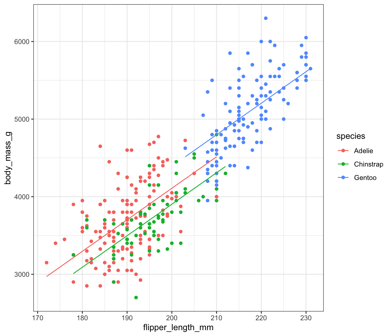
Testing Significance
Let’s introduce some fun R magic!
Show the code
mylm <- lm(body_mass_g ~ species + flipper_length_mm, data = penguins)
anova(mylm, update(mylm, ~ . - species))
Analysis of Variance Table
Model 1: body_mass_g ~ species + flipper_length_mm
Model 2: body_mass_g ~ flipper_length_mm
Res.Df RSS Df Sum of Sq F Pr(>F)
1 329 45843144
2 331 51211963 -2 -5368818 19.265 1.225e-08 ***
---
Signif. codes: 0 '***' 0.001 '**' 0.01 '*' 0.05 '.' 0.1 ' ' 1The update() function takes mylm, uses the full formula (~ .), then removes species.
This is an ESS ANOVA. There is a sig. diff., but it won’t say which group is different!
Note that we can get the same results if we put the predictors in a specific order and use R’s built-in Type 2 ESS algorithm.
Ignore the line for flipper_length_mm, since that’s testing whether adding flipper_length_mmlacement to an empty model improves the results.
Using the code above, verify and explain the following:
- The p-value in the table would be different if we wrote
species + flipper_length_mm.- Note that it would be incorrect.
- The p-value for
flipper_length_mmis different from the one we get in thesummary(mylm)table.
Interaction Terms: Different Intercepts, Different Slopes
We can expand the model above with an interaction term. \[ y = \beta_0 + \beta_1I(Chinstrap) + \beta_2I(Gentoo) + \beta_3 flipper_length_mm + \beta_4I(Chinstrap)flipper_length_mm + \beta_5I(Gentoo)flipper_length_mm \] where \(I(Chinstrap)\) is just shorthand for \(I(species == Chinstrap)\).
This is the same as: \[ y_i = \begin{cases}(\beta_0 + 0) + (\beta_3 + 0) flipper_length_mm& \text{if }\; species == Adelie\\ (\beta_0 + \beta_1) + (\beta_3 + \beta_4) flipper_length_mm& \text{if }\; species == Chinstrap\\(\beta_0 + \beta_2) + (\beta_3 + \beta_5) flipper_length_mm& \text{if }\; species == Gentoo\end{cases} \] In this case, we might as well fit 3 completely different models!
(Except we can test for significance!)
And we’re back to equivalence! Double check the intercepts and slopes for species == "Chinstrap" and species == "Gentoo", using the equations above.
It’s essentially three different models.
Show the code
ggplot(penguins) +
    theme_bw() +
    aes(x = flipper_length_mm, y = body_mass_g, colour = species) +
    geom_point() +
    geom_smooth(method = "lm", se = FALSE, formula = y ~ x)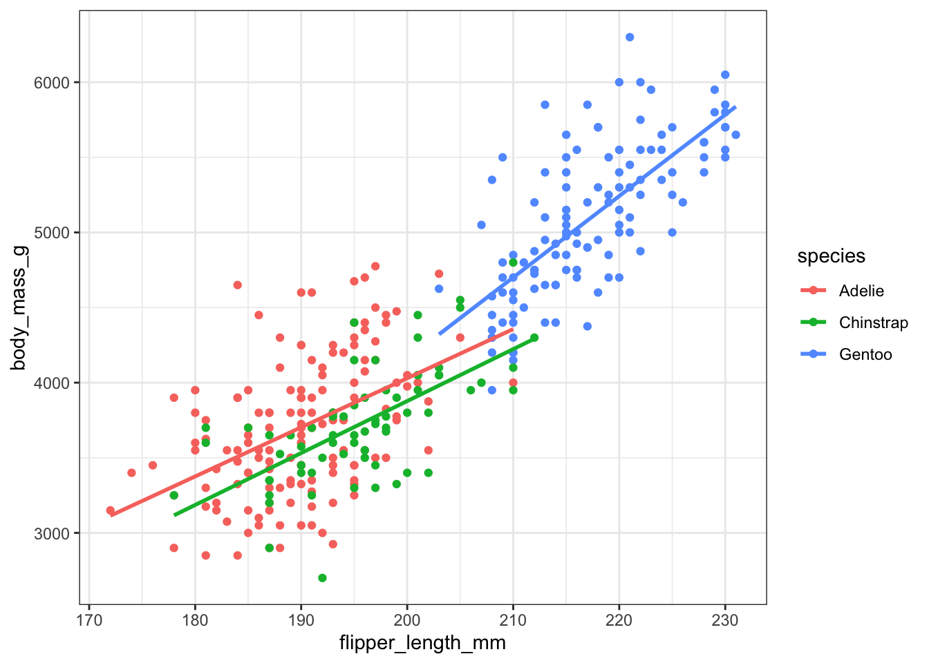
Which “Significance” are we testing?
Show the code
interact_lm <- lm(body_mass_g ~ species * flipper_length_mm, data = penguins)- Significance of
species? - Significance of the interaction?
It depends on the context!
Significance of the Interaction
This is just an ESS for a model with versus without the interaction term:
Show the code
interact_lm <- lm(body_mass_g ~ species * flipper_length_mm, data = penguins)
base_lm <- lm(body_mass_g ~ species + flipper_length_mm, data = penguins)
anova(interact_lm, base_lm)
Analysis of Variance Table
Model 1: body_mass_g ~ species * flipper_length_mm
Model 2: body_mass_g ~ species + flipper_length_mm
Res.Df RSS Df Sum of Sq F Pr(>F)
1 327 44391669
2 329 45843144 -2 -1451475 5.346 0.005193 **
---
Signif. codes: 0 '***' 0.001 '**' 0.01 '*' 0.05 '.' 0.1 ' ' 1The difference in \(SS_{Reg}\) is significant - what does that mean?
ANCOVA
If g is a categorical variable, then:
lm(y ~ g)is a t-test (with equal variance) ifgis binarylm(y ~ g)is an ANOVA ifghas more than 2 categorieslm(y ~ x * g)is an ANCOVA model- ANalysis of COVAriance.
Main idea: Is the covariance (or correlation) between \(x\) and \(y\) different for different categories of \(g\)?
- Only a small extension to ANOVA
- t-test: exactly 2 means
- ANOVA: 2+ means
- ANCOVA: 2+ covariances
Beyond \(x\) and \(g\)
- In the simple cases, we’re doing t-test, ANOVA, or ANCOVA.
- Beyond this, we’re just doing regression, no special names.
- “Controlling for” is a term we might use later.
- Choosing interaction terms is hard.
ggplot2makes parts of it a lot easier.
16.3 Significance of a Group
Output of summary.lm()
The output compares each slope to 0.
- For a categorical predictor, this tests if a category is different from the reference.
There is not an easy built-in way to check significance of a specific group
- For example, we may want to test for equality of intercepts and slopes for Chinstrap and Gentoo penguins, allowing Adelie to have separate values.
- Test for equality of slopes is something covered in the textbook
- Alternative: Change Reference group and use ESS
Changing the reference group
Suppose we want to compare Gentoo and Chinstrap penguins. We can set up our model as: \[
y = \beta_0 + \beta_1I(Gentoo) + \beta_2I(Adelie) + \beta_3flipper_length_mm + \beta_4flipper_length_mmI(Gentoo) + \beta_5flipper_length_mmI(Adelie)
\] where now Chinstrap is the reference group.
We can test \(\beta_1=\beta_4 = 0\) using ESS to test whether body_mass_g versus flipper_length_mm is the same in these two categories.
In R, we need to set up our own dummies to do this.:
penguins$species<- relevel(factor(penguins$species), ref = "Gentoo")
levels(penguins$species)
[1] "Gentoo" "Adelie" "Chinstrap"16.4 Exercises
- Complete the runnable R code above.