Appendix B — Bias/variance of \(\sigma^2\)

Author

Affiliation

Dr. Devan Becker

Wilfrid Laurier University

B.1 Best estimator of \(\sigma^2\)

We saw in the notes that \(E(s^2) = \sigma^2\). Let’s explore why this might not be the best estimator.

We define the MSE of an estimator \(\theta\) as \(E((\theta - \hat\theta^2)^2)\). For the variance, this is \(E((\sigma^2 - s^2)^2)\).

Let’s simulate a bunch of linear models, calculate the standard deviations, and then calculate this quantity.

We’re going to focus on multiplicative bias, and you’ll see why at the end. This means that we’ll focus on estimators of the form \(as^2\).

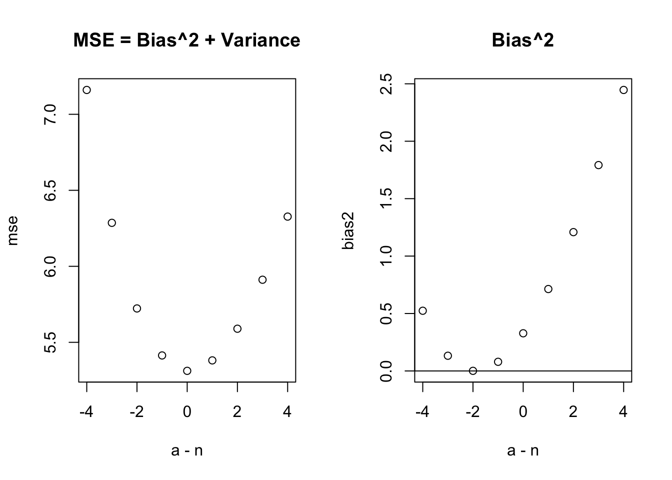
set.seed(2112)

n <- 30
x <- runif(n, 0, 10)
beta0 <- -3
beta1 <- -4
sigma <- 3

reps <- 1000
esst <- double(reps)

for (i in 1:reps) {
    y <- beta0 + beta1*x + rnorm(n, 0, sigma)
    beta1 <- sum((x - mean(x)) * (y - mean(y))) / sum((x - mean(x))^2)
    beta0 <- mean(y) - beta1 * mean(x)
    yhat <- beta0 + beta1 * x
    e <- y - yhat
    esst[i] <- sum(e^2)
}

a <- (n-4):(n+4)
mse <- double(length(a))
bias2 <- double(length(a))
for (i in seq_along(a)) {
    mse[i] <- mean((sigma^2 - esst / a[i])^2)
    bias2[i] <- (sigma^2 - mean(esst / a[i]))^2
}

par(mfrow = c(1,2))
plot(a - n, mse, main = "MSE = Bias^2 + Variance")
plot(a - n, bias2, main = "Bias^2")
abline(h = 0)

From these plots, we see that the lowest MSE, i.e. the lowest value of \(E((\sigma^2 - as^2)^2)\), is at \(a = 1/n\). Note that this corresponds to the MLE of \(\sigma^2\). However, this is a biased estimate, and the unbiased estimate occurs at \(a=1/(n-2)\).

What’s happening here? Shouldn’t unbiased be best? Well, yes, if our criteria is minimizing bias! If we want to minimize \(E((\sigma^2 - \hat\sigma^2)^2)\), we have to account for the variance of the estimator across all possible samples as well!

HWK: Modify the code to show that the bias of the constant model (\(\beta_1 = 0\)) is minimized at \(n-1\), with the MSE being minimized at \(n+1\). It’s bizarre, but that’s how it works!

B.2 Residuals

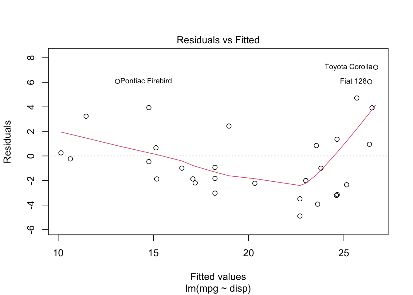
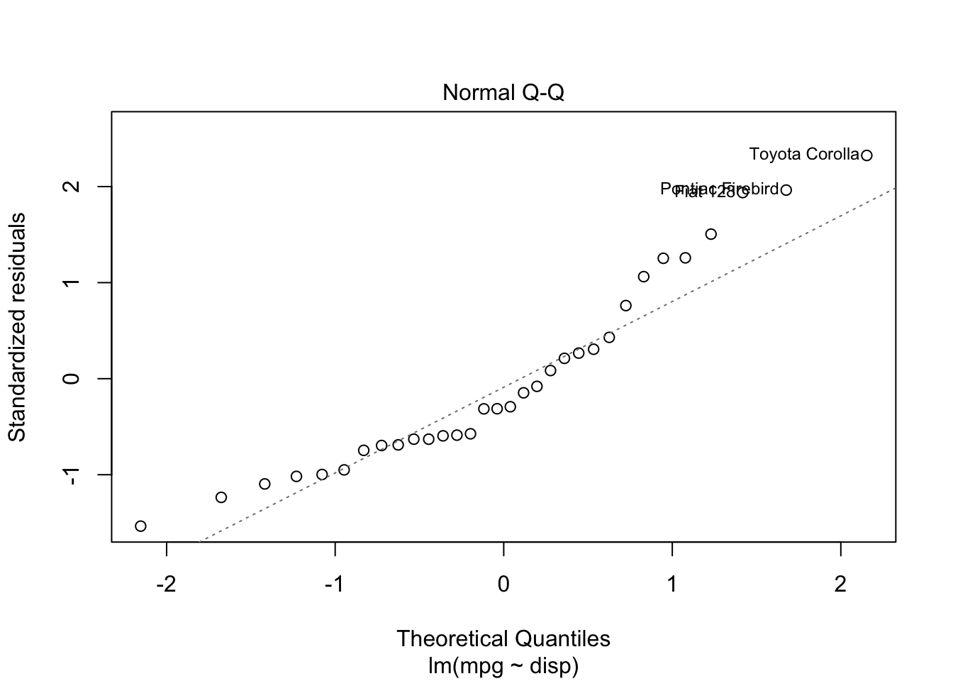
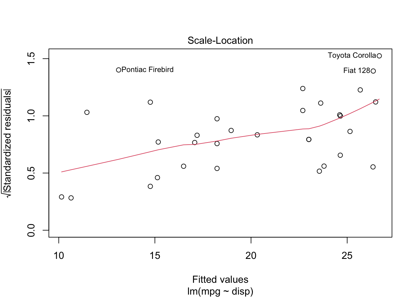
The plot.lm() function makes most of the plots you’ll need.

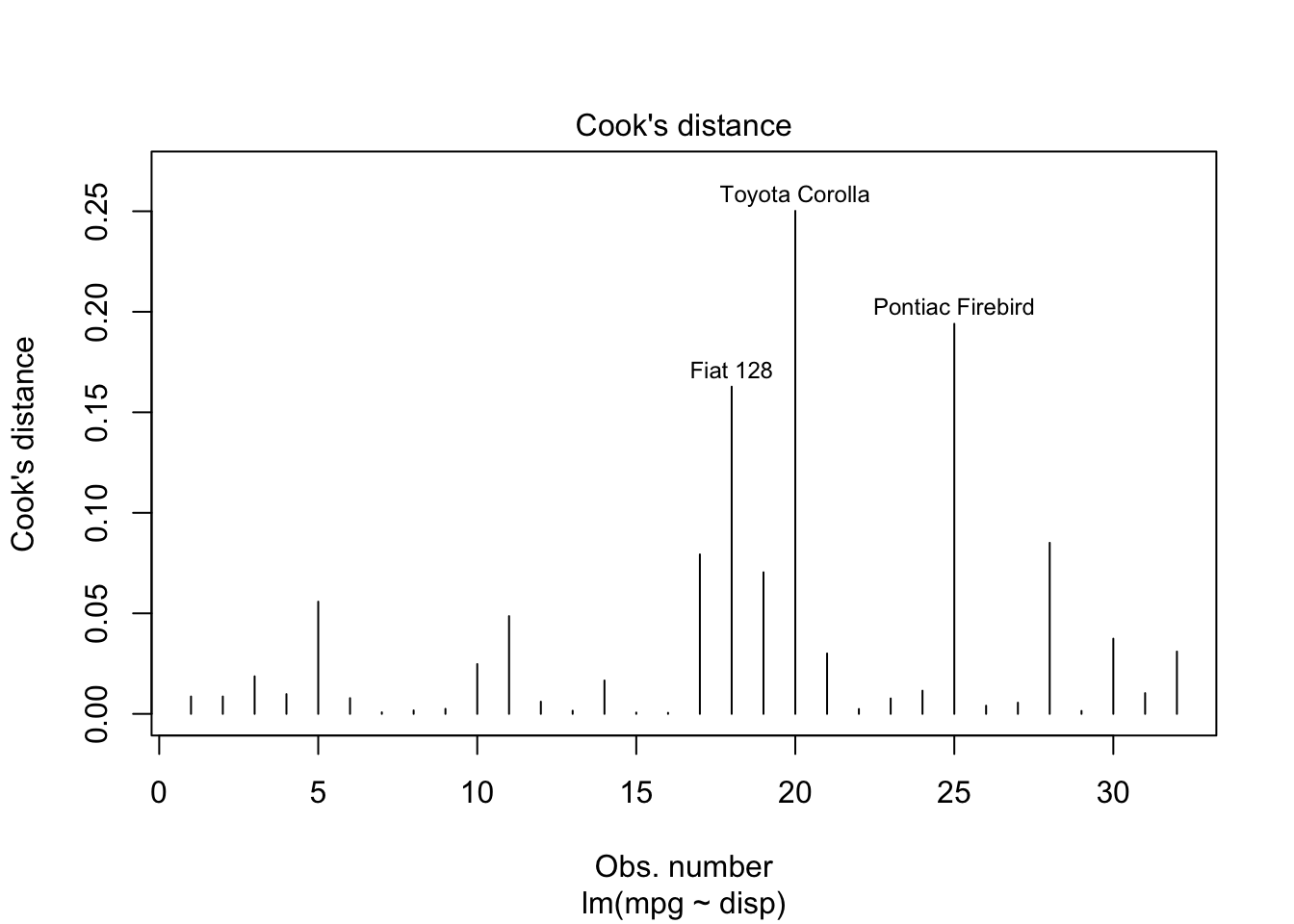
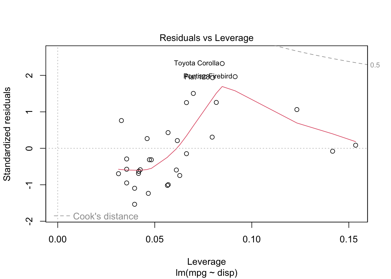
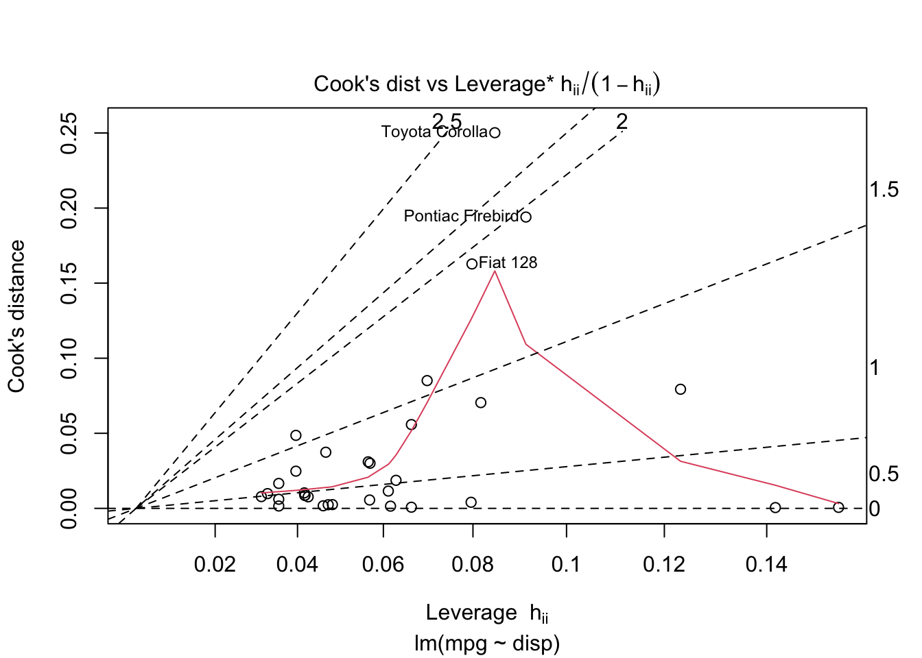
mylm <- lm(mpg ~ disp, data = mtcars)
plot(mylm, which=1:6)

The broom package will be very useful in the future. In particular, the augment() function results in a tidy data frame with columns that are very relevant to our analyses.

library(broom)

head(augment(mylm))

# A tibble: 6 × 9
  .rownames           mpg  disp .fitted .resid   .hat .sigma .cooksd .std.resid
  <chr>             <dbl> <dbl>   <dbl>  <dbl>  <dbl>  <dbl>   <dbl>      <dbl>
1 Mazda RX4          21     160    23.0  -2.01 0.0418   3.29 0.00865     -0.630
2 Mazda RX4 Wag      21     160    23.0  -2.01 0.0418   3.29 0.00865     -0.630
3 Datsun 710         22.8   108    25.1  -2.35 0.0629   3.28 0.0187      -0.746
4 Hornet 4 Drive     21.4   258    19.0   2.43 0.0328   3.27 0.00983      0.761
5 Hornet Sportabout  18.7   360    14.8   3.94 0.0663   3.22 0.0558       1.25 
6 Valiant            18.1   225    20.3  -2.23 0.0313   3.28 0.00782     -0.696

glance(mylm)

# A tibble: 1 × 12
  r.squared adj.r.squared sigma statistic  p.value    df logLik   AIC   BIC
      <dbl>         <dbl> <dbl>     <dbl>    <dbl> <dbl>  <dbl> <dbl> <dbl>
1     0.718         0.709  3.25      76.5 9.38e-10     1  -82.1  170.  175.
# ℹ 3 more variables: deviance <dbl>, df.residual <int>, nobs <int>

anova(mylm)

Analysis of Variance Table

Response: mpg
          Df Sum Sq Mean Sq F value   Pr(>F)    
disp       1 808.89  808.89  76.513 9.38e-10 ***
Residuals 30 317.16   10.57                     
---
Signif. codes:  0 '***' 0.001 '**' 0.01 '*' 0.05 '.' 0.1 ' ' 1

x <- rnorm(1000); qqnorm(x); qqline(x)