12 Non-Linear Relationships with Linear Models
12.1 Non-Linear Relationships
Arbitrarily Shaped Functions
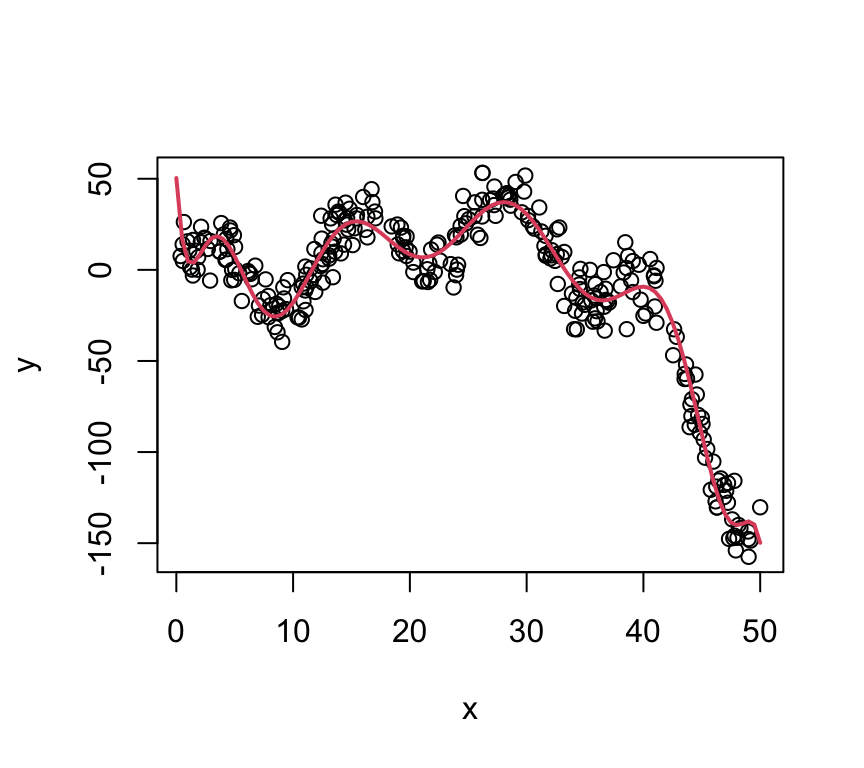
The plot on the right is the function: \[ y = 2 + \frac{1}{5}x^2 - 8\log(x) - 0.005x^3 + 20\sin\left(\frac{x}{2}\right) + \epsilon \]
The twist: The fitted line is just a polynomial model: \(y = \beta_0 + \sum_{j=1}^{12}\beta_jx^j\)
Fitting a Polynomial
To fit a polynomial of order \(k\): \[ y = \beta_0 + \sum_{j=1}^{k}\beta_jx^j + \epsilon \] we can simply fit a linear model to transformed predictors, i.e.: \[ x_1 = x;\; x_2 = x^2;\; x_3 = x^3;\;... \] and we can just fit a linear model as usual!
… that seems too easy?
Choosing Polynomial Order
There are two common options:
- Domain knowledge
- Is there a theoretical reason to use a cubic?
- Reduce prediction error
- Cross-validation or ANOVA, depending on problem.
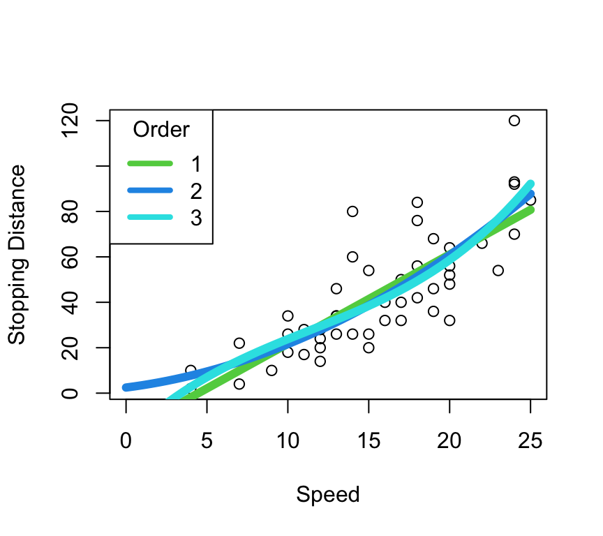
Domain Knowledge: Stopping Distance
The stopping distance is theoretically proportional to the square of the speed.
- A line might fit
- Fits poorly at 0 (negative stopping distances for positive speed?)
- A quadratic fits better?
- A cubic does something funky at 0.
Choosing Order with ANOVA
Show the code
X <- data.frame(dist = cars$dist, x1 = cars$speed, x2 = cars$speed^2,
    x3 = cars$speed^3, x4 = cars$speed^4)
lm(dist ~ ., data = X) |> anova()
Analysis of Variance Table
Response: dist
Df Sum Sq Mean Sq F value Pr(>F)
x1 1 21185.5 21185.5 92.5775 1.716e-12 ***
x2 1 528.8 528.8 2.3108 0.1355
x3 1 190.4 190.4 0.8318 0.3666
x4 1 336.5 336.5 1.4707 0.2316
Residuals 45 10297.8 228.8
---
Signif. codes: 0 '***' 0.001 '**' 0.01 '*' 0.05 '.' 0.1 ' ' 1In this situation, Sequential Sum-of-Squares makes sense! (Disagrees with theory, though. Go with theory.)
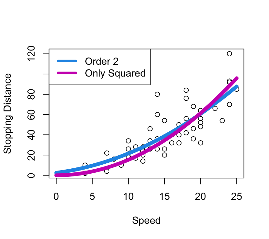
Stopping Distance \(\propto\) Speed\(^2\)
A second order polynomial is: \[ y = \beta_0 + \beta_1x + \beta_2x^2 \]
The implied model is: \[ y = \beta_2x^2 \]
Unconventional ESS
Show the code
X <- data.frame(dist = cars$dist, x1 = cars$speed, x2 = cars$speed^2,
    x3 = cars$speed^3, x4 = cars$speed^4)
m1 <- lm(dist ~ x1 + x2, data = X)
m2 <- lm(dist ~ -1 + x2, data = X)
anova(m2, m1)
Analysis of Variance Table
Model 1: dist ~ -1 + x2
Model 2: dist ~ x1 + x2
Res.Df RSS Df Sum of Sq F Pr(>F)
1 49 11936
2 47 10825 2 1111.2 2.4123 0.1006Not a significant difference in models, so go with simpler one: \(y = \beta_2x^2\)
- This is highly specific to this situation - see cautions later.
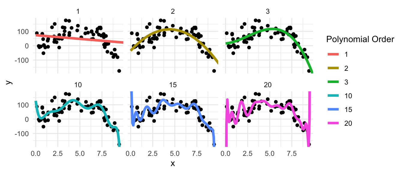
Polynomial Models will Overfit!
True model: \(f(x) = 2 + 25x + 5x^2 - x^3\) (cubic), Var(\(\epsilon\)) = 40
Multiple Regression Polynomial Models
A full polynomial model of order 2 with two predictors is: \[ y = \beta_0 + \beta_1x_1 + \beta_2x_2 + \beta_{11}x_1^2 + \beta_{22}x_2^2 + \beta_{12}x_1x_2 \] In R this can be specified as:
Show the code
lm(y ~ (x1 + x2)^2)- This is why you can’t use
y ~ x + x^2to get a polynomial model - R tries to interpret this as a model specification rather than a transformation. - We’ll learn more about interactions and transformations in the next few lectures.
12.2 Cautions about Polynomials
Lower Order Terms
Unless there’s a strong physical reason,
- \((ax - b)^2\) is the model, not \(\beta_0 + \beta_1x + \beta_{11}x^2\)
Orders higher than 3 are rarely jutified
Recall the interpretation of a slope:
- A one unit increase in \(x\) is associated with a \(\beta_1\) unit increase in \(y\).
- This interpretation fails in quadratrics, and fails spectacularly in higher orders.
See splines for more flexibility
Extrapolation is Fraught with Peril
Unless you have the true order (you don’t), polynomials diverge almost immediately.
Show the code
shiny::runGitHub(repo = "DB7-CourseNotes/TeachingApps",
subdir = "Apps/polyFit")poly() uses orthogonal polynomials
Show the code
betas <- replicate(1000,
    coef(lm(y ~ poly(x, 2, raw = TRUE),
         data = data.frame(x = runif(30, 0, 10),
            y = (x - 2)^2 + rnorm(30, 0, 10)))))
plot(t(betas))
After squaring, cubing, etc., each column of X is transformed to be orthogonal to the previous.
- Takes care of transformations for you when using
predict(). - The
coef()function is useless. - Mean-centering also helps!
Orthogonal Polynomials
Show the code
x <- sort(runif(60, 0, 10))
par(mfrow = c(2,3))
for(i in 1:3) {
    plot(x, poly(x, 3, raw = TRUE)[,i])
}
for(i in 1:3) {
    plot(x, poly(x, 3, raw = FALSE)[,i])
}
12.3 Should I Use a Polynomial?
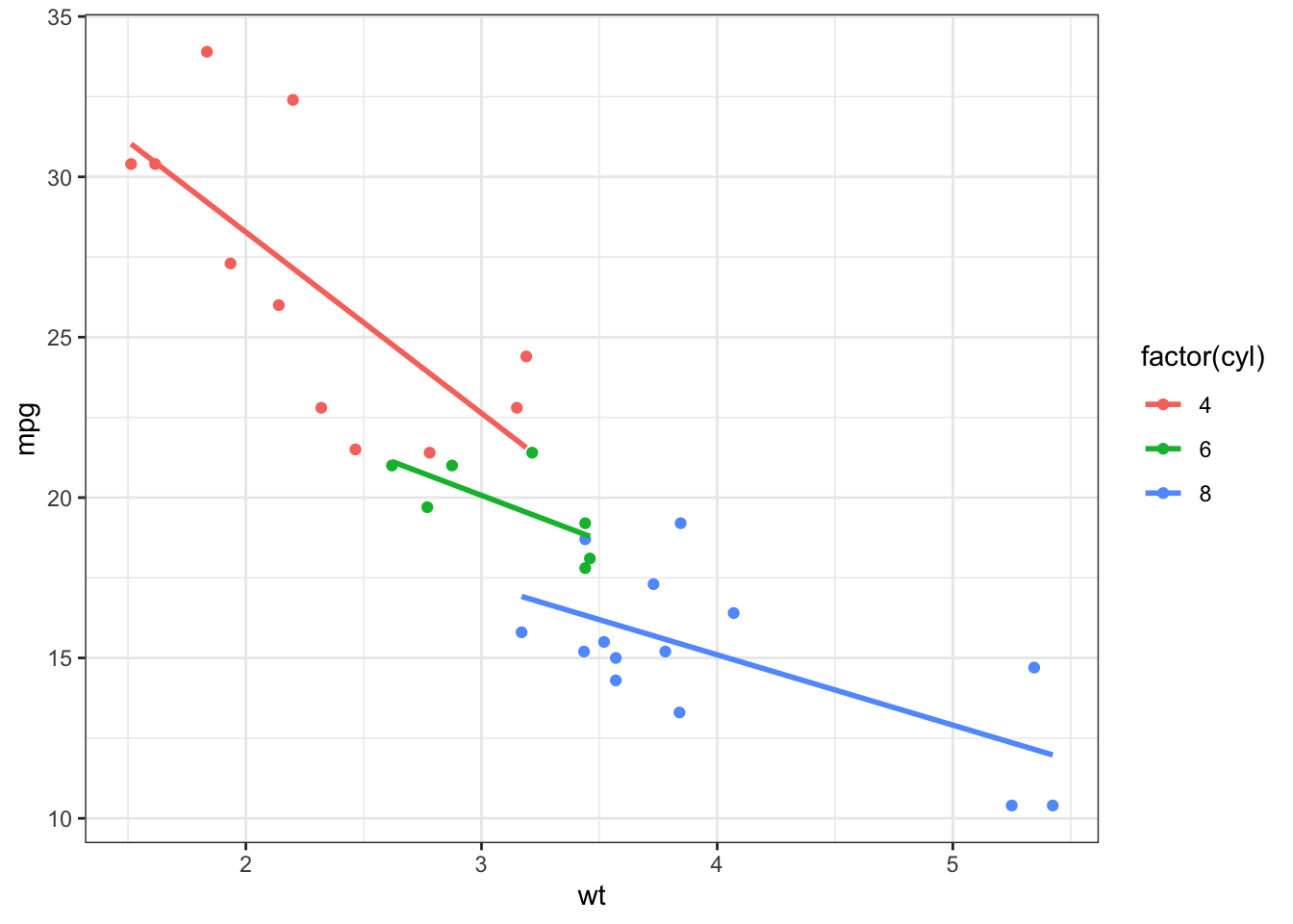
Example: mtcars
[code]
Play around with the polynomial order in the following code to try and get a good fit! (For fun, also try a degree 17 polynomial.) Then, reveal the solution below.
Note that you can run this code right here - you don’t need to use your own computer! This is magical!
Solution
A polynomial model is not the best model here! The following plot shows three related linear models (which we’ll learn about later), demonstrating that it is linear but there’s a hidden grouping!
Closing Notes: Linear Models are fine with non-linear trends
The formula \(y_i = \beta_0 + \beta_1x_{i1} + \beta_2x_{i2} + ... + \epsilon_i\) doesn’t care how \(x\) is defined.
- \(x_{i2} = x_{i1}^2\) works as if \(x_{i1}\) and \(x_{i2}\) are just two predictors.
- \(x_{i2} = \log(x_{i1})\) is fine too!
- \(x_{i2} = \log(x_{i1}) + \exp(x_{i3})\tan(1)\)? Sure, why not!
- \(x_{i2} = \log(\beta_1x_{i1})\) is a total no-go.
- Linear models are linear in the parameters.