shiny::runGitHub(
    repo = "DB7-CourseNotes/TeachingApps",
    subdir = "Apps/multico"
)15 Multicollinearity
15.1 The Problem
The Problem with Multicollinearity
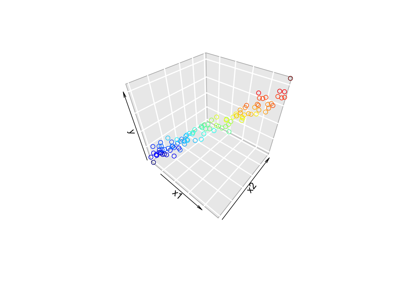
- Multiple regression fits a hyperplane
- If the points form a “tube”, an infinite number of hyperplanes work.
- Rotate plane around axis of tube.
Consequences of the Problem
High cor. in \(X\) \(\implies\) high cor. in \(\hat{\underline\beta}\).
- Many combos of \(\hat{\underline\beta}\) are equally likely
- No meaningful CIs
Show the code
set.seed(2112)
replicate(1000, {
    y <- 0 + 4*x1 + 3*x2 + rnorm(n, 0, 5)
    coef(lm(y ~ x1 + x2))[-1]
}) |>
    t() |>
    plot(xlab = expression(hat(beta)[1]),
        ylab = expression(hat(beta[2])),
        main = "Estimated betas for correlated\npredictors, many samples")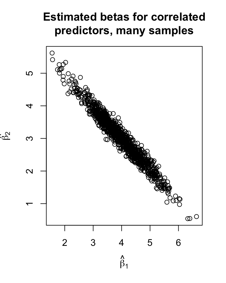
Another Formulation of the Problem
Consider the model \(y_i = \beta_0 + \beta_1x_{i1} + \beta_2x_{i2} + \epsilon_i\), where \(x_{i1} = a + bx_{i2} + z_i\) and \(z_i\) represents some extra uncertainty.
Fitting the model, we could:
- Set \(\hat\beta_1\) to 0, let \(x_2\) model all of the variance.
- Set \(\hat\beta_2\) to 0, let \(x_1\) model all of the variance.
- Set \(\hat\beta_1\) to any value, solve for \(\hat\beta_2\).
- Basically the same results regardless of what \(\hat\beta_1\) is chosen as.
In other words, the parameter estimates are not unique (or nearly not unique).
The Source of the Problem
\[ \hat{\underline{\beta}} = (X^TX)^{-1}X^TY,\quad V(\hat{\underline{\beta}}) = (X^TX)^{-1}\sigma^2 \]
- If two columns of \(X\) are linearly dependent, then \(X^TX\) is singular.
- Constant predictor value (linearly dependent with column of 1s).
- Unit change (one column for Celcius, one for Fahrenheit).
- If two columns of \(X\) are nearly linearly dependent, then some elements of \((X^TX)^{-1}\) are humungous.
- Two proxy measure for the same thing (e.g., daily high and low temperatures).
- Nearly linear transformation (e.g., polynomial or BMI)
Detecting the Problem
The variance-covariance matrix of \(X\) can be useful: \[ Cov(X) = \begin{bmatrix} 0 & 0 & 0 & 0 & \cdots\\ 0 & V(X_1) & Cov(X_1, X_2) & Cov(X_1, X_3) & \cdots\\ 0 & Cov(X_1, X_2) & V(X_2) & Cov(X_2, X_3) & \cdots\\ 0 & Cov(X_1, X_3) & Cov(X_2, X_3) & V(X_3) & \cdots\\ \vdots & \vdots & \vdots & \vdots & \ddots \end{bmatrix} \] Why are the first column/row 0?
Plotting \(V(X)\)
Show the code
library(palmerpenguins); library(GGally)
ggcorr(penguins)
Warning in ggcorr(penguins): data in column(s) 'species', 'island', 'sex' are
not numeric and were ignored
Detecting the Problem: \(V(\hat{\underline\beta})\)
Unfortunately, the var-covar matrix is hard to get from R.
- We can look at the SE column of the summary output!
- Very very very much not conclusive.
- The Variance Inflation Factor
The Variance Inflation Factor
We can write the variance of each estimated coefficeint as: \[ V(\hat\beta_i) = VIF_i\frac{\sigma^2}{S_{ii}} \] where \(S_{ii} = \sum_{k=1}^n(x_{ki} - \bar{x_i})^2\) is the “SS” for the \(i\)th column of \(X\).
- If there is no “Variance Inflation”, then VIF = 1
- “Inflation” comes from the idea of rotating a plane around a “tube”.
- Also interpreted as a measure of linear dependence with other columns of \(X\).
Interpreting the Variance Inflation Factor
Consider a regression of \(X_i\) against all other predictors.
- The \(R^2\) measures how well the other predictors can model \(X_i\)
- Label this \(R_i^2\) to indicate it’s the \(R^2\) for \(X_i\) against other columns.
- Important: We’re not considering \(\underline y\) at all!
The VIF is calculated as: \[ VIF_i = \frac{1}{1 - R_i^2} \]
- If \(R_i^2=0\), then \(VIF_i = 1\)
- If \(R_i^2\rightarrow 1\), then \(VIF_i \rightarrow \infty\)
Penguins VIF in R
Show the code
library(car) # vif() function
bogy_mass_lm <- lm(
    formula = body_mass_g ~ flipper_length_mm + bill_length_mm + bill_depth_mm,
    data = subset(penguins, species == "Chinstrap")
)
vif(bogy_mass_lm)
flipper_length_mm bill_length_mm bill_depth_mm
1.541994 1.785702 2.092955 Bad VIF in R
Show the code
x1 <- runif(n, 0, 10)
x2 <- 2 + x1 + runif(n, -1, 1)
y <- 0 + 4*x1 + 3*x2 + rnorm(n, 0, 5)

mylm <- lm(y ~ x1 + x2)
vif(mylm)
x1 x2
23.39082 23.39082 Rule of thumb: VIF > 10 is a bad thing. 5 < VIF < 10 is worth looking into.
Show the code
scatter3D(x1, x2, y, bty = "g", colkey = FALSE,
    xlab = "x1", ylab = "x2", zlab = "y")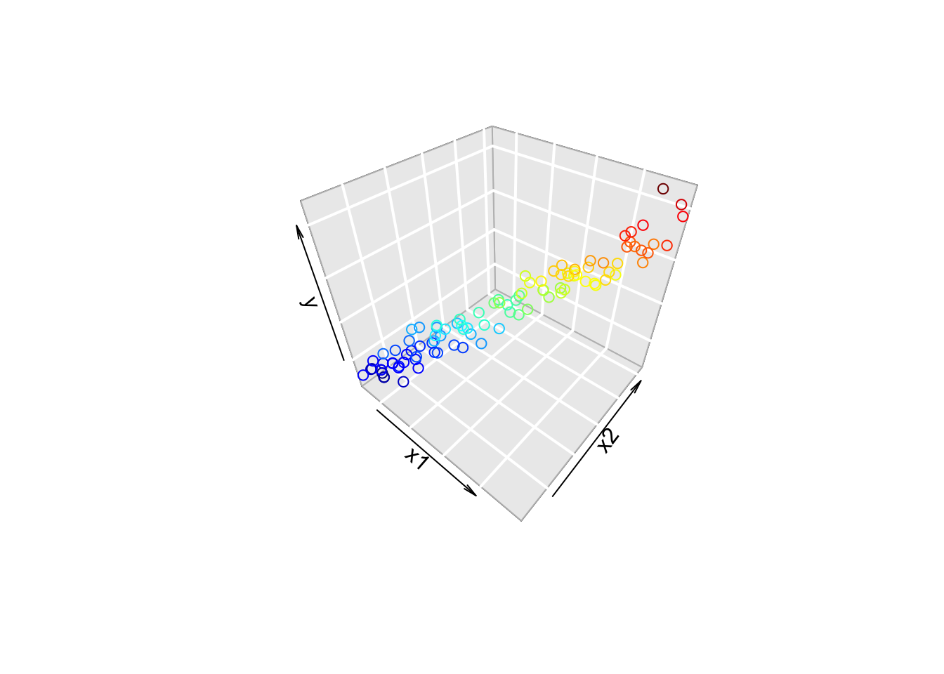
Try changing the code until the VIF is less than 10. What do you notice about the plot?
Change the variables that say “Change me!” and see what happens. Note: You can hold the “Shift” button and hit “Enter” to run the code. You can hold shift and hit enter repeatedly to do a sort of psuedo-simulation (notice how VIF also has a sampling distribution!).
Limitation: This is just one of many, many, many ways in which predictors can be correlated.
15.2 Will Scaling Fix the Problem
Scaling the Predictors
If we subtract the mean and divide by the sd, some of the correlation goes away.
- This is actually kinda bad - we’ve hidden some multicollinearity from ourselves!
If \(Z\) is the standardized version of \(X\), then \[ Cor(X) = Z^TZ/(n-1) \]
If \(Z\) is the mean-centered version of \(X\), then \[ Cov(X) = Z^TZ/(n-1) \]
15.3 Fixing The Problem
One way to fix the problem
Don’t.
We can’t get good estimates of the \(\hat\beta\)s, but we can still get good predictions.
- This only works if the new values are in the same “tube” as the others.
- If the multicollinearity is real, what estimates do you expect?
- Without a controlled experiment, there isn’t a good way to estimate the effect of \(X_1\) on it’s own!
Removing predictors
If two predictors are measuring the same thing, then just include one?
- This might lose some information!
- It also might not!
- The estimated \(\beta\) won’t be meaningful.
- Inferences will be difficult.
- There might be a good reason to choose one predictor (or transform them).
- Example: Height and weight are correlated, but BMI might be more useful to medical researchers.
- BMI is highly fraught.
- Example: If you have Celcius and Fahrenheight…
- Example: Height and weight are correlated, but BMI might be more useful to medical researchers.