14  Modelling with Transformations

Author
Affiliation

Dr. Devan Becker

Wilfrid Laurier University

Published

2024-07-03

14.1 Introduction

The Trees Data

data(trees)
trees$Diam <- trees$Girth / 12
trees$Girth <- NULL
head(trees)
  Height Volume      Diam
1     70   10.3 0.6916667
2     65   10.3 0.7166667
3     63   10.2 0.7333333
4     72   16.4 0.8750000
5     81   18.8 0.8916667
6     83   19.7 0.9000000

From the help file:

  • Girth” is actually the diameter, in inches
    • Renamed Diam, transformed to feet
  • Height is in feet
  • Volume of the timber (usable wood) (cubic feet)

Goal: Model the volume of the tree as a function of Height and Diameter.

DIY

The course notes include some starter code (that can be run in browser). Can you fit a better model than the basic multiple linear regression?

Get in groups, use pen and paper to record the important parts of the transformations you try.

Hint: what’s the Volume of a cylinder?

My Attempts

In the following, I’ll try a couple different models.

Note that I’ve made the output smaller for the slides - you want to look at more than just these values!

Multiple Linear Regression

data(trees)
trees$Diam <- trees$Girth / 12
trees$Girth <- NULL
base_lm <- lm(Volume ~ Diam + Height, data = trees)
summary(base_lm)$coef |> round(4)
            Estimate Std. Error t value Pr(>|t|)
(Intercept) -57.9877     8.6382 -6.7129   0.0000
Diam         56.4979     3.1712 17.8161   0.0000
Height        0.3393     0.1302  2.6066   0.0145
summary(base_lm)$adj.r.squared
[1] 0.9442322

Multiple Linear Regression - Plots

Attempt 1: Logs

Notice that the model \(E(y_i) = \beta_1x_{i1}^2x_{i2}\) is equivalent to: \[ \ln(E(y_i)) = \ln(\beta_1) + 2\ln(x_{i1}) + \ln(x_{i2}) \]

full_log_lm <- lm(log(Volume) ~ log(Height) + log(Diam), data = trees)
summary(full_log_lm)$coef |> round(4)
            Estimate Std. Error t value Pr(>|t|)
(Intercept)  -1.7049     0.8819 -1.9332   0.0634
log(Height)   1.1171     0.2044  5.4644   0.0000
log(Diam)     1.9826     0.0750 26.4316   0.0000
summary(full_log_lm)$adj.r.squared
[1] 0.976084

Attempt 1 Residual Plots

Alternative 2: log(y)

Let’s try not logging the x-values

y_log_lm <- lm(log(Volume) ~ Height + Diam, data = trees)
summary(y_log_lm)$coef |> round(4)
            Estimate Std. Error t value Pr(>|t|)
(Intercept)   0.1026     0.2153  0.4764   0.6375
Height        0.0164     0.0032  5.0508   0.0000
Diam          1.7435     0.0790 22.0569   0.0000
summary(y_log_lm)$adj.r.squared
[1] 0.9661964

Attempt 2 Residual Plots

Box-Cox?

  • Box-Cox says something between 0 and 1, closer to 0.
  • What could we round to?
library(MASS)
boxcox(lm(Volume ~ Height + Diam, data = trees))

Using the Box-Cox Parameter: Sqrt

y_sqrt_lm <- lm(sqrt(Volume) ~ Height + Diam, data = trees)
summary(y_sqrt_lm)$coef |> round(4)
            Estimate Std. Error t value Pr(>|t|)
(Intercept)  -2.7700     0.5094 -5.4375    0e+00
Height        0.0358     0.0077  4.6589    1e-04
Diam          4.8591     0.1870 25.9828    0e+00
summary(y_sqrt_lm)$adj.r.squared
[1] 0.9740084

Using the Box-Cox Parameter: Quarter Power

y_quarter_lm <- lm(I(Volume^(1/4)) ~ Height + Diam, data = trees)
summary(y_quarter_lm)$coef |> round(4)
            Estimate Std. Error t value Pr(>|t|)
(Intercept)   0.5108     0.1057  4.8318        0
Height        0.0085     0.0016  5.3258        0
Diam          1.0235     0.0388 26.3699        0
summary(y_quarter_lm)$adj.r.squared
[1] 0.9753826

What About Transforming \(x\) only?

poly_lm <- lm(Volume ~ poly(Height, 2) + poly(Diam, 2), data = trees)
summary(poly_lm)$coef |> round(4)
                 Estimate Std. Error t value Pr(>|t|)
(Intercept)       30.1710     0.4802 62.8290   0.0000
poly(Height, 2)1  13.1319     3.1368  4.1864   0.0003
poly(Height, 2)2   0.4266     2.9584  0.1442   0.8865
poly(Diam, 2)1    80.2382     3.1323 25.6167   0.0000
poly(Diam, 2)2    15.2171     2.9632  5.1354   0.0000
summary(poly_lm)$adj.r.squared
[1] 0.9735436

Quadratic Polynomial Plots

Polynomials of Order 8? (\(R^2\) = 0.9864, \(R^2_{adj}\) = 0.9708)

My Solution

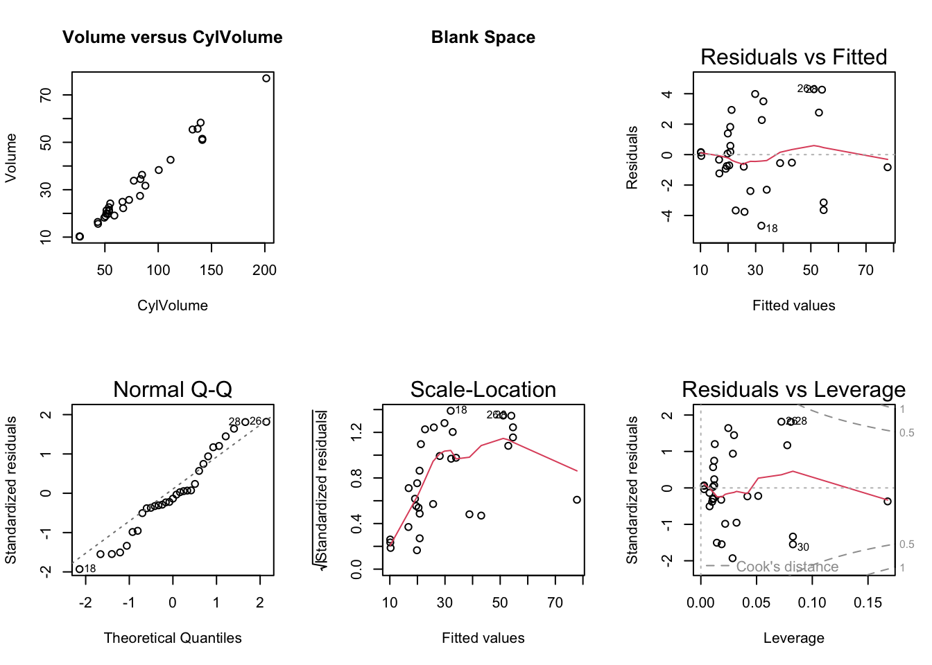
Let CylVolume be the volume of the cylinder defined by Height and Diam, \(V = \pi (d/2)^2h\).

The model is \(Volume_i = \beta_1CylVolume_i + \epsilon_i\), where \(\beta_1\) is the proportion of an ideal cylinder that is actual usable wood.

trees$CylVolume <- pi * (trees$Diam/2)^2 * trees$Height
cyl_lm <- lm(Volume ~ -1 + CylVolume, data = trees)
summary(cyl_lm)$coef |> round(4)
          Estimate Std. Error t value Pr(>|t|)
CylVolume   0.3865      0.005 77.4365        0
summary(cyl_lm)$adj.r.squared
[1] 0.994856

CylVolume Plots

par(mfrow = c(2, 3))
plot(Volume ~ CylVolume, data = trees,
    main = "Volume versus CylVolume")
plot(1, main = "Blank Space", bty = "n", xaxt = "n", yaxt = "n",
    xlab = "", ylab = "", pch = "")
plot(cyl_lm)

Some Closing Thoughts

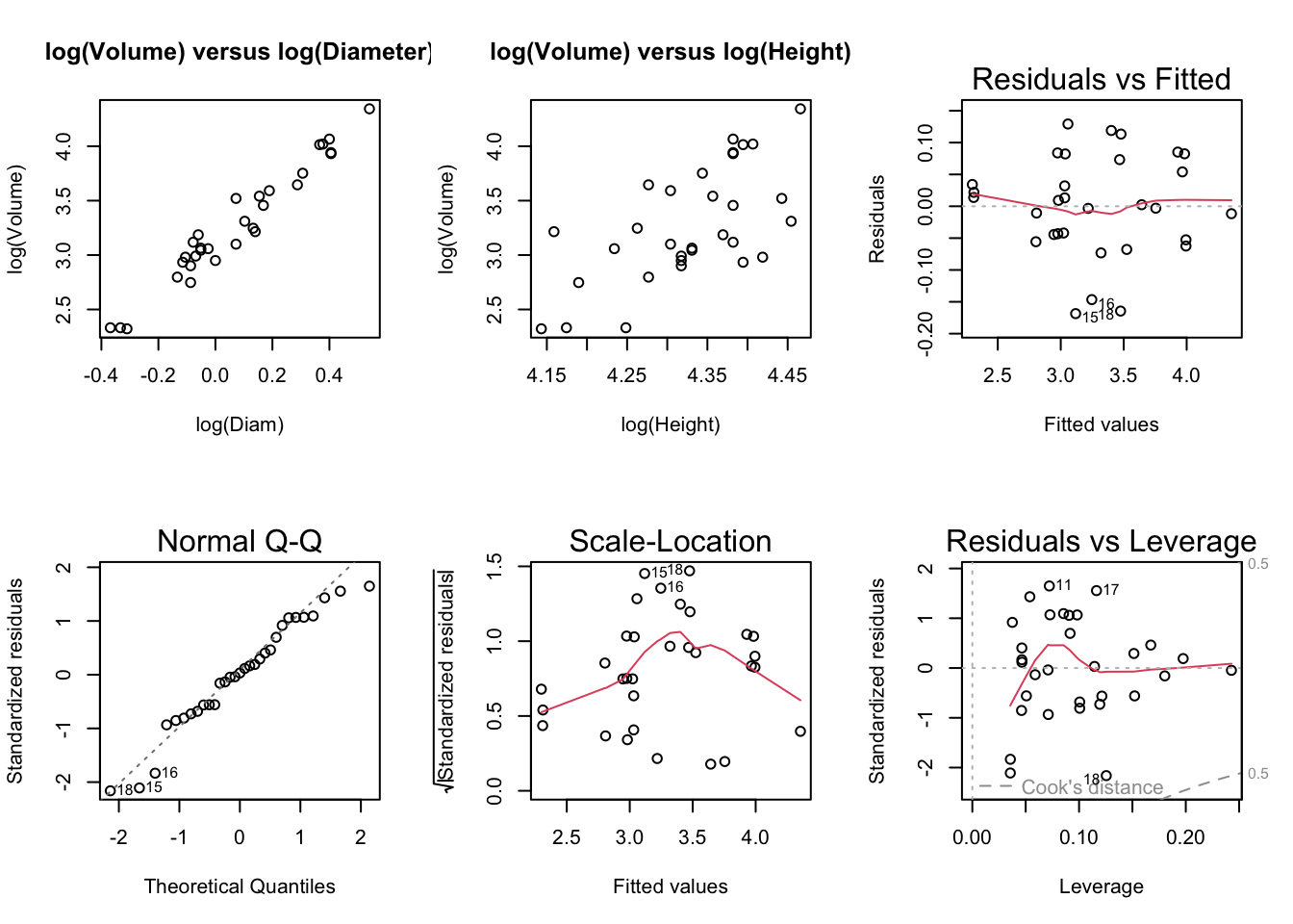
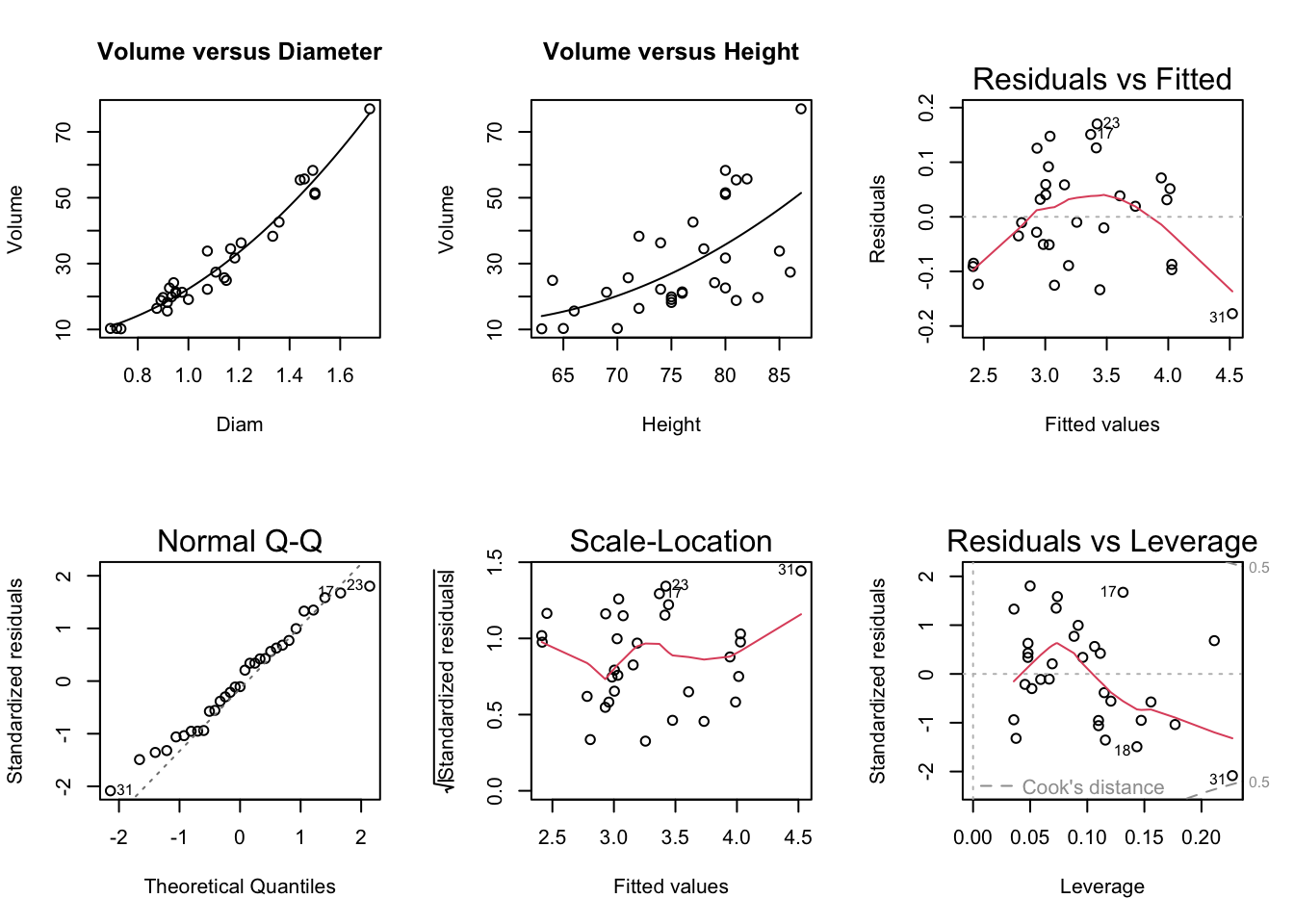
  • Using ln(y) ~ ln(x) made the \(R^2\) slightly better, even though plots looked similar.
    • Plots looked slightly better for full log, though.
  • We were using log just to make the relationship linear.
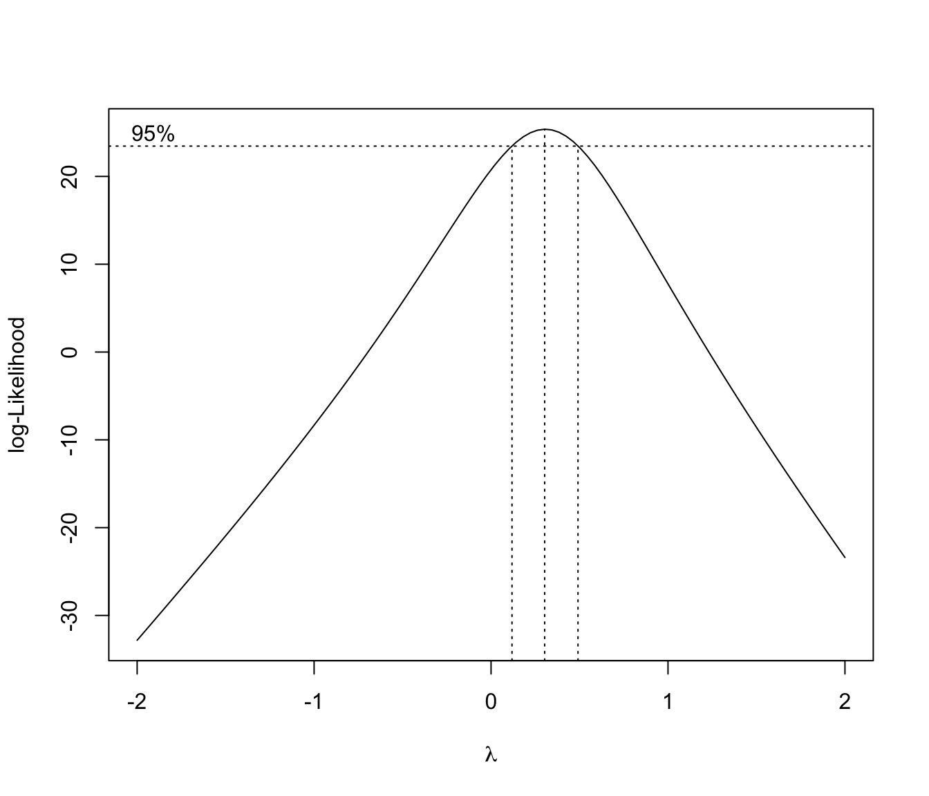
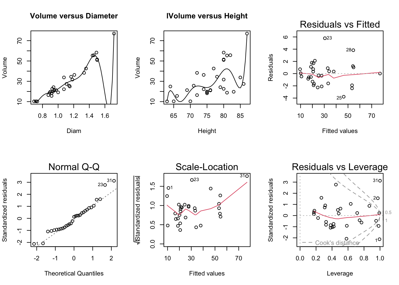
    • Box-Cox told us to use sqrt or quarter power instead - result was better!
  • Very interestingly, models that chose powers of \(x\) chose 1 for Height, 2 for Diam…
  • Trees are not perfect cylinders.
    • However, a cylinder model fits best and with fewer parameters!!!

In conclusion, always think through the problem before blindly modelling.

Note that the best model in this case used our knowledge of the physical problem, and this happened to correspond to the best fitting model. This isn’t always the case! It is very common that we’ll have to choose between a model that fits well and a model that matches our understanding of the world, and this is not an easy choice!