Our estimates of \(\beta_0\) and \(\beta_1\) are very close to the truth!
Now, let’s generate new data a bunch of times and see if our estimate of the variance of \(\hat\beta_1\) is accurate. This is not a proof, just a demonstration.
In the code below, I’m also keeping track of \(\hat\beta_0\) from each sample. This will be useful later.
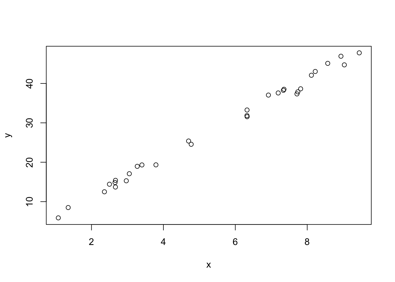
In this example, we know the data generating process (dgp), so these randomly generated values are samples from the population.
As we know, the standard error is the variance of the estimator over all possible samples from the population. We only took 1000, but that’s probably close enough to infinity to draw the sampling distribution.
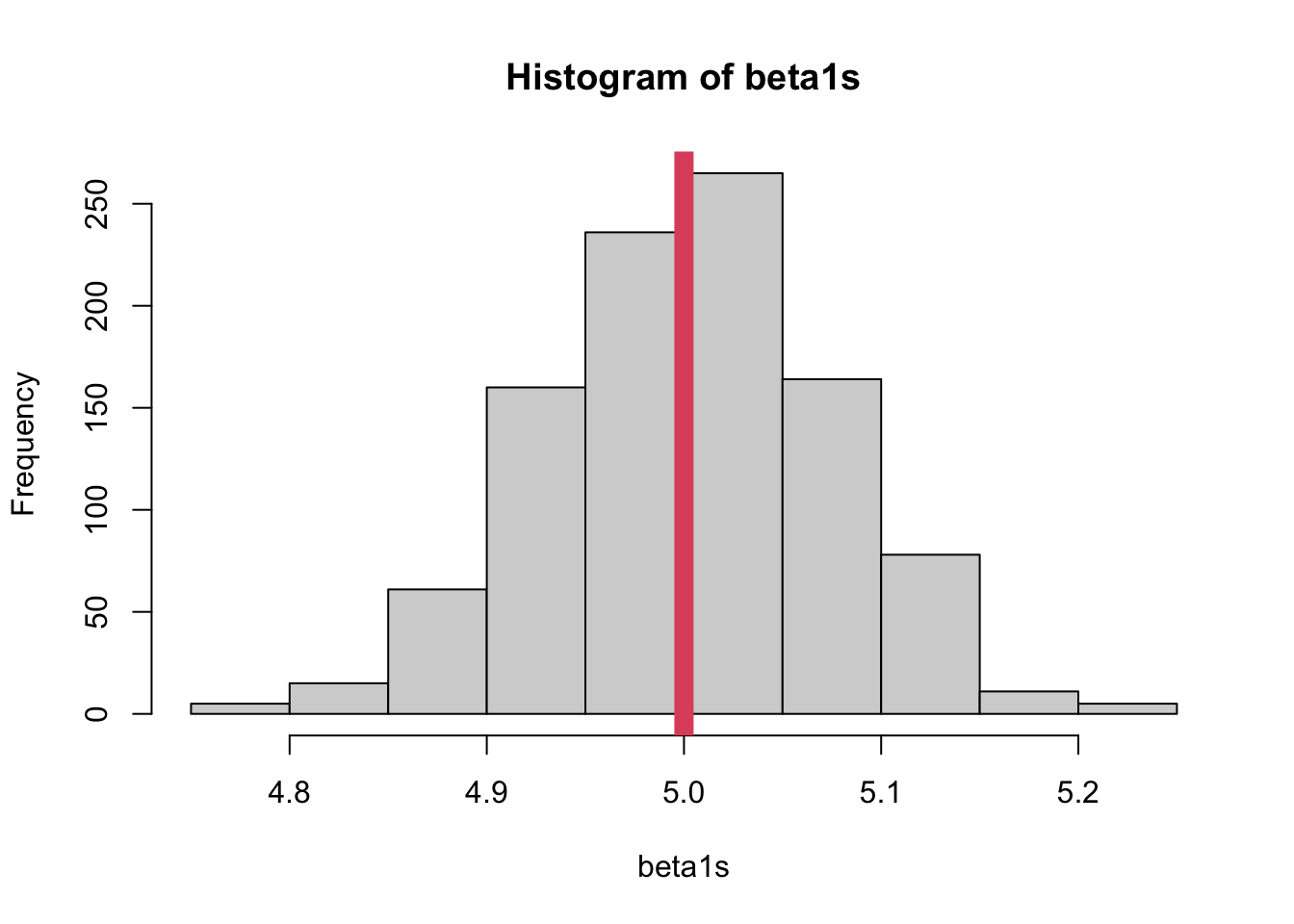
hist(beta1s)abline(v =5, col =2, lwd =10) # true value of beta
As you can see, \(\hat\beta_1\) is unbiased and has some variance (at this stage, there’s nothing to compare this variance to so we can’t really call it “large” or “small”).
Let’s use this to calculate an 89% Confidence Interval!
The empirical and the theoretical CIs line up pretty well! However, the sample CI is fundamentally different. The sample CI is centered at the estimated value, and we expect it to contain the true population value 89% of the time!
We practically never know the actual DGP, so this is just a demonstration that the math works.
Note that we treated \(\underline x\) as if it were fixed. The value \(S_{XX}\) will be different for different \(\underline x\), and we don’t make any assumptions about what distribution \(\underline x\) follows.
A.1 Analysis of Variance
The code below demonstrates how the ANOVA tables are calculated.
        Source df         SS          MS
1   Regression  1 4809.33809 4809.338089
2        Error 28   30.93852    1.104947
3 Total (cor.) 30 4840.27661  161.342554
This is equivalent to what R’s built-in functions do!
anova(lm(y ~ x, data = mydata))
Analysis of Variance Table

Response: y
          Df Sum Sq Mean Sq F value    Pr(>F)
x          1 4809.3  4809.3  4352.5 < 2.2e-16 ***
Residuals 28   30.9     1.1
---
Signif. codes:  0 '***' 0.001 '**' 0.01 '*' 0.05 '.' 0.1 ' ' 1
A.2 Dependence and Centering
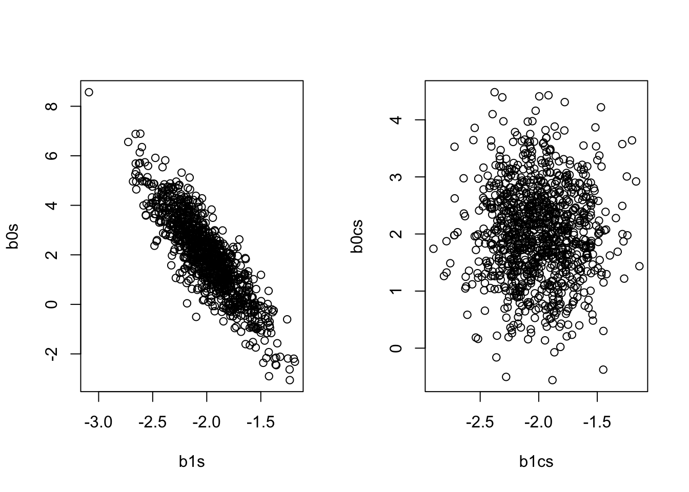
Something not touched on in class is that \(cov(\hat\beta_0, \hat\beta_1)\) is not 0! This should be clear from the formula got \(\hat\beta_0\), which is \(\hat\beta_0 = \bar y - \hat\beta_1\bar x\).
The code below repeats what we did before, but with higher variance to better demonstrate the problem.
It also records the estimates based on centering\(\underline x\). Notice how the formula for \(\hat\beta_0\) is no longer dependent on \(\hat\beta_1\) if the mean of \(\underline x\) is 0!