20 Classification
20.1 Logistic Regression
Goal: Predict a 1
- Response: 0 or 1
- Predictions: probability of a 1?
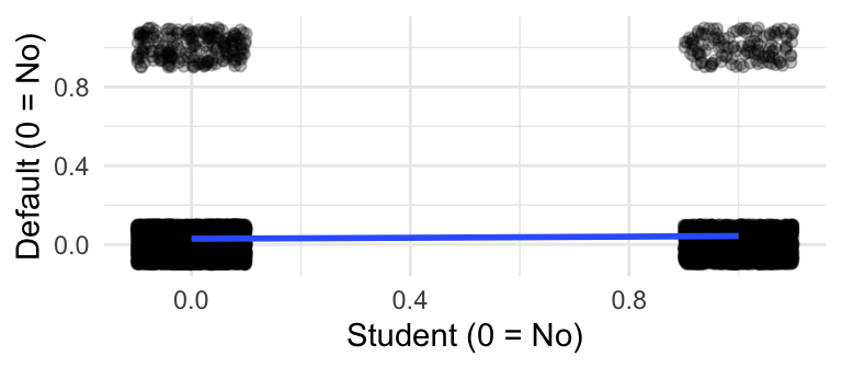
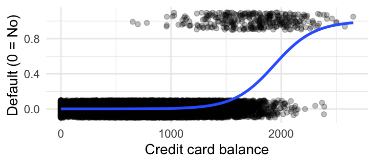
Why Not Linear Regression?
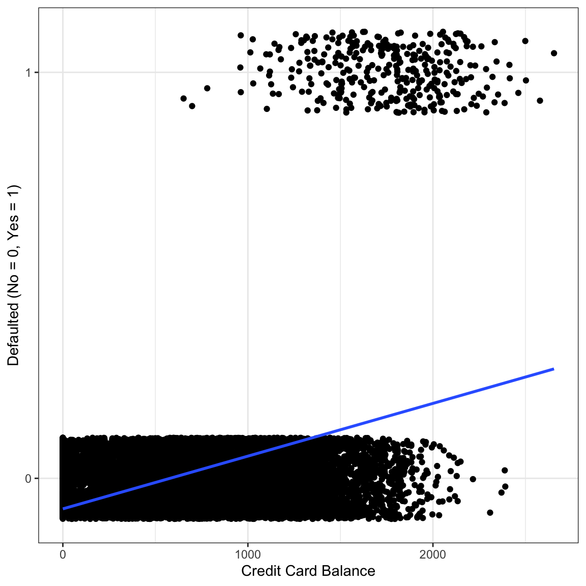
The plot on the right shows Default versus Credit Card Balance (with jittering).
- “Default” is 0 for No, 1 for Yes
- Dummy encoding for the response
- Linear model predicts negative values!
- Also, values above 1.
- What could the slope possibly represent???
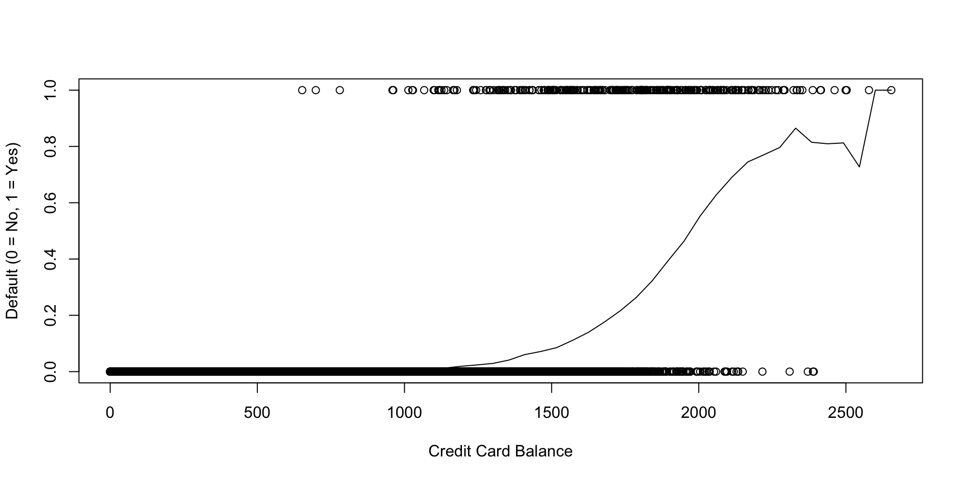
The mean of y at each value of x
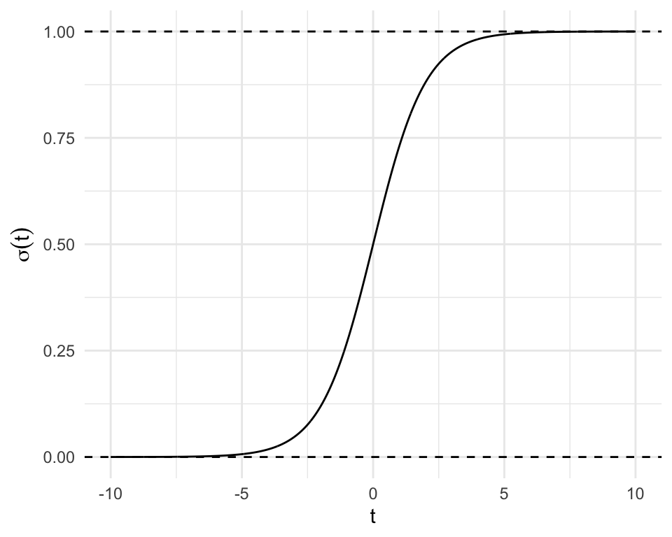
The Logistic Function - A Sigmoid
If \(t\in\mathbb{R}\), then \[ \sigma(t) = \dfrac{\exp(t)}{1 + \exp(t)}\in[0,1] \] where \(\sigma(\cdot)\) is the logistic function.
Logistic Function - Now with Parameters
\[ \sigma(\beta_0 + \beta_1 t) \]
#| standalone: true
#| viewerHeight: 600
#| viewerWidth: 800

xseq <- seq(-10, 10, 0.05)
sigma <- function(t) exp(t)/(1 + exp(t))

input <- list(b0 = 0, b1 = 1)

ui <- fluidPage(
    sidebarPanel(
        sliderInput("b0", "Intercept B_0", -5, 5, 0, 0.1, animate = list(interval = 100)),
        sliderInput("b1", "Slope B_1", -5, 5, 1, 0.1, animate = list(interval = 100))
    ),
    mainPanel(plotOutput("plot"), )
)

server <- function(input, output) {
    output$plot <- renderPlot({
        yseq <- sigma(input$b0 + input$b1 * xseq)
        plot(yseq ~ xseq,
            xlim = c(-10, 10),
            ylim = c(0, 1),
            ylab = bquote(sigma (beta[0] *" + " * beta[1] * t)),
            xlab = "t",
            type = "l")
    })
}

shinyApp(ui = ui, server = server)
Logistic Function - Now with Parameters Estimated from DATA
\[\begin{align*} \eta(x_i) &= X\underline{\beta}\\ p_i &= \sigma(\eta(x_i))\\ \implies \log\left(\frac{p_i}{1-p_i}\right) &= X\underline{\beta} \end{align*}\]
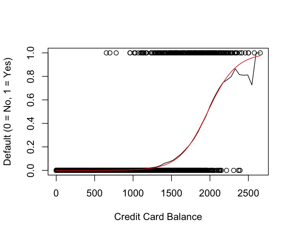
\(\eta(x_i) = -10.65 + 0.0054\cdot\text{balance}_i\)
Logistic Regression
- The response is 0 or 1 (no or yes, don’t default or default, etc.)
- The probability of a 1 increases according to the sigmoid function.
- The linear predictor is \(\eta(x_i) = \beta_0 + \beta_1x_{i1} + \beta_2x_{i2} + \cdots\)
- The probability of class 1 is \(P(\text{class }1 | \text{predictors}) = \sigma(\eta(x_i))\)
- Instead of normality assumptions, we use a binomial distribution.
It’s just one step away from a linear model!
Interpreting Slope Parameters
- General structure: “For each one unit increase in \(x_i\), some function of \(y_i\) changes by some function of \(\beta\)”.
- For logistic regression:
- One unit increase in \(x_i\), \(\log\left(\frac{p(x_i)}{1-p(x_i)}\right)\) increases by \(\beta\).
- The odds are \(\frac{p(x_i)}{1-p(x_i)}\).
- “1 in 5 people with odds of 1/4 will default.”
- \(\beta\) is the change in log odds for a one unit increase.
- “log odds ratio”.
Odds Ratios
Consider the one-predictor example.
\[ \eta(x_i) = \beta_0 + \beta_1x_{i1}\text{ and }\eta(x_i + 1) = \beta_0 + \beta_1x_i + \beta_1\text{, }\therefore \eta(x_i + 1) - \eta(x_i) = \beta \]
The logg odds ratio is defined as \[ \log(OR) = \log\left( \frac{p(x_i + 1)}{1 - p(x_i + 1)} \middle/ \frac{p(x_i)}{1 - p(x_i)}\right) \] Using \(\eta(x_i) = \log\left(\frac{p(x_i)}{1-p(x_i)}\right)\), show that \(\log(OR) = \beta_1\)
The Loss Function
For all observations:
- If \(y_i = 0\), we want \(p(x_i)\) to be as low as possible.
- Maximize \(1 - P(Y_{i} = 1|\beta_0,\beta_1,X)\)
- If \(y_i = 1\), we want \(p(x_i)\) to be as high as possible.
- Maximize \(P(Y_{i} = 1|\beta_0,\beta_1,X)\)
These can be combined as: \[ \prod_{i:y_{i} = 0}\left(1 - P(Y_{i} = 1|\beta_0,\beta_1,X)\right)\prod_{i:y_i=1}P(Y_i = 1|\beta_0,\beta_1,X) \] which is equivalent to: \[ \prod_{i=1}^n(1 - P(Y_{i} = 1|\beta_0,\beta_1,X))^{1 - Y_i}P(Y_i = 1|\beta_0,\beta_1,X)^{Y_i} \]
Which is NOT just the sum of squared errors!
Unlike linear regression, there’s no closed form for \(\hat{\beta}_0\) and \(\hat\beta_1\); we need numerical methods.
Examples: Two different predictors in the Default data
\[ \eta(x_i) = -3.5 + 0.5\cdot\text{student} \]
Odds of a student defaulting are \(\exp(0.5)\approx1.65\) times as high as a non-student.
\[ \eta(x_i) = -10.65 + 0.005\cdot\text{balance} \]
Each extra dollar of CC balance increases odds of defaulting by a factor of 1.005.
The scale of the predictors matters.
Odds versus Probabilities
“The odds of a student defaulting are \(\exp(0.5)\approx1.65\) times as high as a non-student.”
\[ \frac{P(\text{default} | \text{student} = 1)}{1 - P(\text{default} | \text{student} = 1)} \biggm/ \frac{P(\text{default} | \text{student} = 0)}{1 - P(\text{default} | \text{student} = 0)} = 1.65 \]
This cannot be solved for \(P(\text{default} | \text{student} = 1)\)!
\[ P(\text{default} | \text{student} = 1) = \dfrac{\exp(\eta(x_i))}{1 + \exp(\eta(x_i))} \approx 0.047 \]
Multiple Linear Logistic Regression
- Predictors can be multicollinear, confounded, and have interactions.
- Logistic is just Linear on a transformed scale!
- We do not look for transformations of the response.
- It’s already a transformation of the response \(p_i(x_i)\)!
- We do look for transformations of the predictors!
- Sigmoid + Polynomial is where the real fun is.
Errors in Logistic Regression: Deviance
- All “errors” are either \(p(x_i)\) or \(1 - p(x_i)\).
- i.e., distances are measured form either 0 or 1.
Instead, we use the deviance.
- If \(p(x_i)\) were the true probability in a binomial distribution, what’s the probability of the observed value (0 or 1)?
- In other words, \(P(Y_i = 1| \beta_0, \beta_1, X)\) and \(1 - P(Y_i = 1| \beta_0, \beta_1, X)\) are the residuals!
- The residual we use depends on what the response is. If \(y_i = 0\), the residual is \(P(Y_i = 1 | \beta_0, \beta_1, X)\)
- This is used more broadly in Generalized Linear Models (GLMs). Logistic Regression is one of many GLMs.
- In other words, \(P(Y_i = 1| \beta_0, \beta_1, X)\) and \(1 - P(Y_i = 1| \beta_0, \beta_1, X)\) are the residuals!
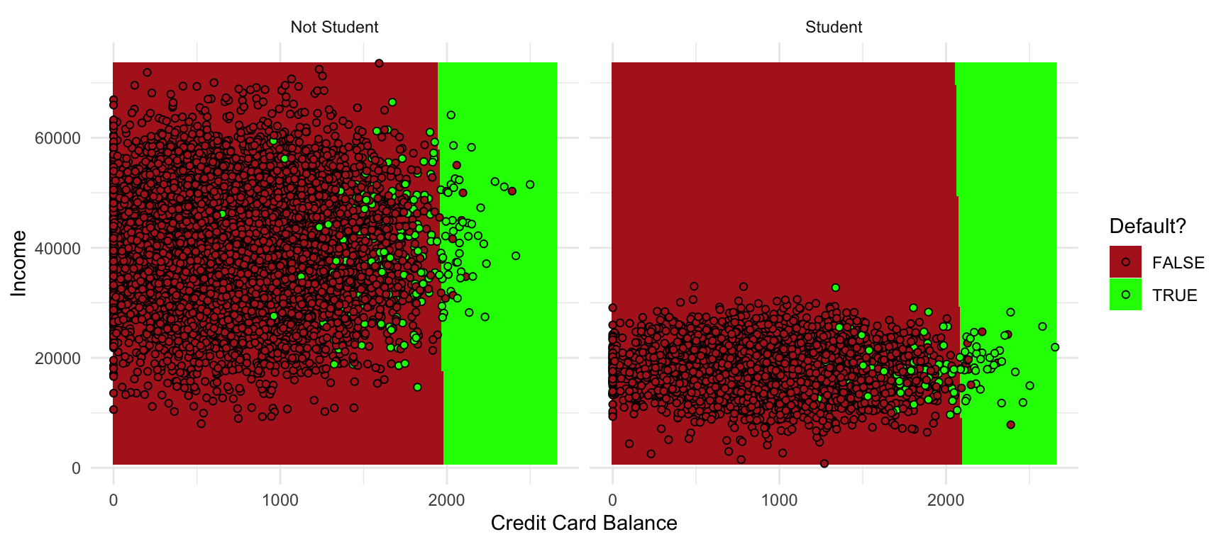
Logistic Decision Boundaries
\[ P(\text{defaulting} | \eta(x_i)) > p \implies a + bx_1 + cx_2 + dx_3 > e \]
for some (linear) hyperplane \(a + bx_1 + cx_2 + dx_3\) and some value \(e\).
- Choosing \(p=0.5\) is standard, but other thresholds can be chosen.
- Cancer example: want to be more admissive of false positives
- Would rather operate and be wrong than falsely tell the patient that they’re healthy!
- Cancer example: want to be more admissive of false positives
Predictions - Just Plug it In!
| Intercept | Student | Balance | Income | |
|---|---|---|---|---|
| \(\beta\) | -10.09 | -0.65 | 0.0057 | 0.000003 |
We can make a prediction for a student with $2,000 balance and $20,000 income: \[\begin{align*} \eta(x) &= \beta_0 + \beta_1\cdot 1 + \beta_2\cdot 2000 + \beta_3\cdot 20000 \approx 0.0178\\ &\\ P(\text{defaulting} | x) &= \dfrac{\exp(\eta(x))}{1 + \exp(\eta(x))} \approx \dfrac{\exp(0.0178)}{1 + \exp(0.0178)} \approx 0.504\\ &\\ &P(\text{defaulting} | x) > 0.5 \implies \text{Predict Default} \end{align*}\]
Standard Errors: It’s complicated
We don’t have an estimate like \(\hat\beta = (X^TX)^{-1}X^TY\). We had to resort to numerical methods.
There is a closed form for \(V(\hat\beta)\) and a way to test significance, but they’re beyond the scope of this course.
- Relies on likelihoods, which we avoided in this course.
- You can assume significance tests in R output are correct.
20.2 Classification Basics
Goal: Predict a Category
- Binary: Yes/no, success/failure, etc.
- Categorical: 2 or more categories.
- A.k.a. qualitative, but that’s a social science word.
In both: predict whether an observation is in category \(j\) given its predictors. \[ P(Y_i = j| x = x_i) \stackrel{def}{=} p_j(x_i) \]
Classification Confusion
Confusion Matrix: A tabular summary of classification errors.
| True Pay (\(\cdot 0\)) | True Def (\(\cdot 1\)) | |
|---|---|---|
| Pred Pay (\(0 \cdot\)) | Good (00) | Bad (01) |
| Pred Def (\(1 \cdot\)) | Bad (10) | Good (11) |
- Two ways to be wrong
- Two ways to be right
- Different applications have different needs
Accuracy: \(\dfrac{\text{Correct Predictions}}{\text{Number of Predictions}} =\frac{00 + 11}{00 + 01 + 10 + 11}\)
Is “Accuracy” Good?
Task: Predict whether a person has cancer
(In this made up example, 0.02% of people have cancer).
| True Healthy | True Cancer | |
|---|---|---|
| Pred. Healthy | Save a Life | Lose a Life |
| Pred. Cancer | Expensive/Invasive | All good |
- Easy: 99.8% accuracy.
- Always guess “Not Cancer”
- Very Hard: 99.82% accuracy.
The Confusion Matrix for Default Data
| True Payment | True Default | |
|---|---|---|
| Pred Payment | 9627 | 228 |
| Pred Default | 40 | 105 |
- This model: 97.32% accuracy.
- Naive model: always predict “Pay” - 96.67% accuracy!
Other important measures (not on exam):
- Sensitivity: \(\dfrac{\text{True Positives}}{\text{All Positives in Data}} = \dfrac{9627}{9627 + 40} = 99.58%\) (Naive: 100%)
- Specificity: \(\dfrac{\text{True Negatives}}{\text{All Negatives in Data}} = \dfrac{105}{105 + 228} = 31.53\) (Naive: 0%)
Logistic Regression in R
The residual plots are the same as before:
The predictions can either be on the logit scale (type = "link", the default) or on the response scale (probabilities).
Regularization is often used with logistic regression (in python’s scikit-learn package, Ridge regularization is used by default without warning the user).