Appendix I — Regression with Categorical Predictors
Author
Affiliation
Dr. Devan Becker
Wilfrid Laurier University
Published
2024-04-22
I.1 Regression as a t-test
When we do regression against a dummy variable, we are actually just doing a t-test.
A regression models the mean of \(y\) for each value of \(x\).
A one-unit increase in \(X\) is the difference between 0 and 1.
The slope is the difference in means.
We assume constant variance
Same variance at \(x=0\) and \(x=1\).
A t-test has a df of \(n-1\), so does a regression with just one predictor.
Show the code
# Note that I need the var.equal=TRUE to match the assumptions of regression.t.test(mpg ~ am, data = mtcars, var.equal =TRUE)
    Two Sample t-test

data:  mpg by am
t = -4.1061, df = 30, p-value = 0.000285
alternative hypothesis: true difference in means between group 0 and group 1 is not equal to 0
95 percent confidence interval:
 -10.84837  -3.64151
sample estimates:
mean in group 0 mean in group 1
       17.14737        24.39231
Show the code
lm(mpg ~ am, data = mtcars) |>summary()
Call:
lm(formula = mpg ~ am, data = mtcars)

Residuals:
    Min      1Q  Median      3Q     Max
-9.3923 -3.0923 -0.2974  3.2439  9.5077

Coefficients:
            Estimate Std. Error t value Pr(>|t|)
(Intercept)   17.147      1.125  15.247 1.13e-15 ***
am             7.245      1.764   4.106 0.000285 ***
---
Signif. codes:  0 '***' 0.001 '**' 0.01 '*' 0.05 '.' 0.1 ' ' 1

Residual standard error: 4.902 on 30 degrees of freedom
Multiple R-squared:  0.3598,    Adjusted R-squared:  0.3385
F-statistic: 16.86 on 1 and 30 DF,  p-value: 0.000285
The two outputs have the exact same test statistic and p-value!
I.2 Categorical Predictors as ANOVA
In order for R to recognize a variable as a dummy variable, we need to tell it that the values should be interpreted as a factor. This is a very particular data type:
Every observation is one level of the categorical variable.
Every observation can only be one level of that categorical variable
E.g., a car can’t have 4 cylinders and 6 cylinders
There are a finite number of possible categories.
Unless we specify, R assumes that the unique values that it sees constitutes all the possible categories. In other words, it won’t let us ask about cars with 5 cylinders because we’re making a factor variable with 4, 6, and 8 as the observed values.
Show the code
anova(aov(mpg ~factor(cyl), data = mtcars))
Analysis of Variance Table

Response: mpg
            Df Sum Sq Mean Sq F value    Pr(>F)
factor(cyl)  2 824.78  412.39  39.697 4.979e-09 ***
Residuals   29 301.26   10.39
---
Signif. codes:  0 '***' 0.001 '**' 0.01 '*' 0.05 '.' 0.1 ' ' 1
Show the code
summary(lm(mpg ~factor(cyl), data = mtcars))
Call:
lm(formula = mpg ~ factor(cyl), data = mtcars)

Residuals:
    Min      1Q  Median      3Q     Max
-5.2636 -1.8357  0.0286  1.3893  7.2364

Coefficients:
             Estimate Std. Error t value Pr(>|t|)
(Intercept)   26.6636     0.9718  27.437  < 2e-16 ***
factor(cyl)6  -6.9208     1.5583  -4.441 0.000119 ***
factor(cyl)8 -11.5636     1.2986  -8.905 8.57e-10 ***
---
Signif. codes:  0 '***' 0.001 '**' 0.01 '*' 0.05 '.' 0.1 ' ' 1

Residual standard error: 3.223 on 29 degrees of freedom
Multiple R-squared:  0.7325,    Adjusted R-squared:  0.714
F-statistic:  39.7 on 2 and 29 DF,  p-value: 4.979e-09
The overall test of significance has an F-value of 39.7 and a p-value of 4.979x10\(^{-9}\)
But what is up with the summary.lm() output? Why do we have a row labelled factor(cyl)6??
I.3 Coding Dummy Variables (what factor is actually doing)
When we have multiple variables, we set one aside as the “reference” category. For a factor variable with \(k\) categories, we set up \(k-1\) new variables to denote category membership. For example:
4 is the reference category for cyl. If all the new dummy variables that we create are all 0, then the car must be 4 cylinders.
We set up a dummy variable for 6 cylinders, which is a column with a 1 if the car has 6 cylinders and a 0 otherwise. This is what’s labelled as factor(cyl)6 in the output.
This can be denoted \(I(cyl == 6)\).
Similarly, we have factor(cyl)8 = \(I(cyl == 8)\).
Consider the model \(y = \beta_0 + \beta_1I(cyl == 6) + \beta_2I(cyl == 8)\).
With this setup, the intercept represents the estimate for 4 cylinder cars, \(\beta_1\) represents the difference in 4 and 6 cylinder cars, while \(\beta_2\) represents the difference in 4 and 8 cylinder cars (you can find the difference between 6 and 8 by doing the right math).
From model.matrix(), we can see this in action:
Show the code
cbind(model.matrix(mpg ~factor(cyl), data = mtcars), cyl =cbind(mtcars$cyl)) |>head(12)
The advantage of having all three in one is that we can test for significance easily!
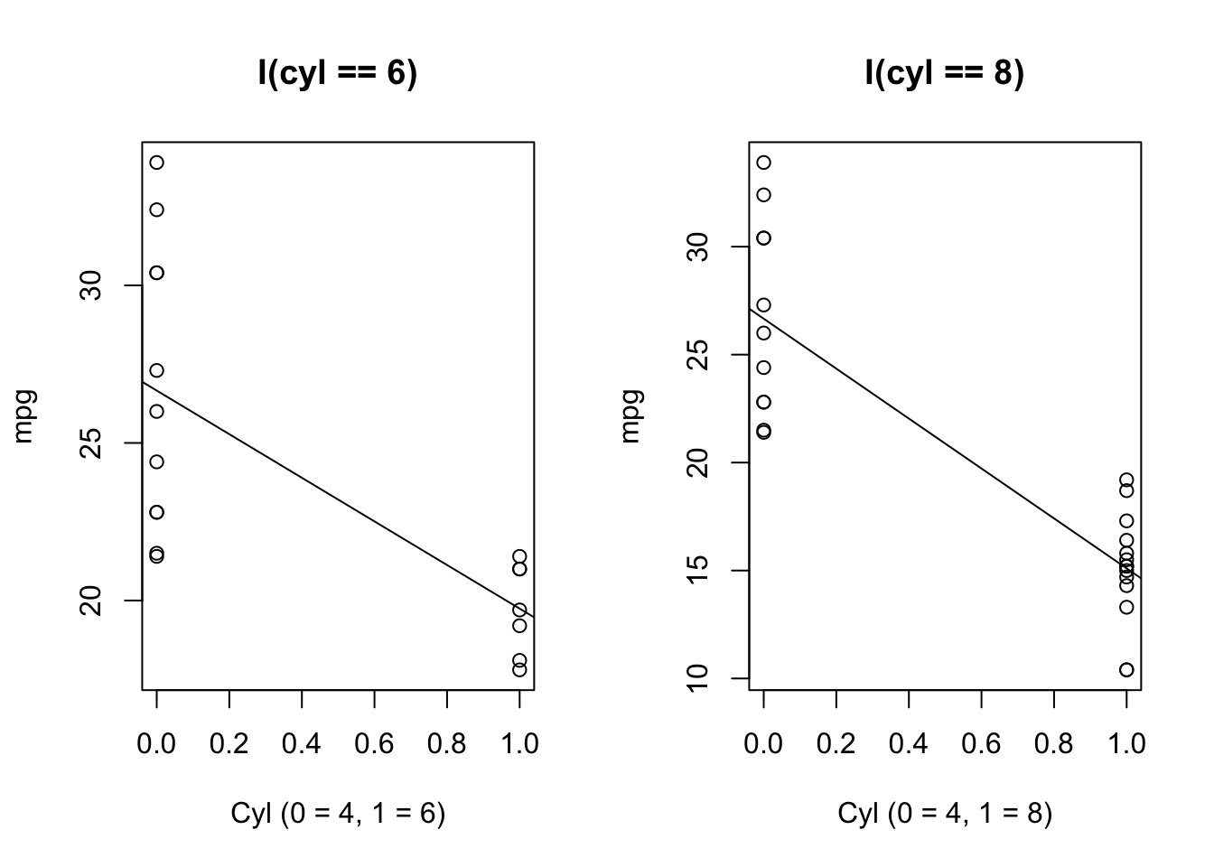
One way (a bad way) to visualize this is to treat \(I(cyl ==6)\) and \(I(cyl==8)\) as separate variables:
Show the code
par(mfrow =c(1,2))plot(mpg ~I(as.numeric(factor(cyl)) -1), data =subset(mtcars, cyl %in%c(4,6)),xlab ="Cyl (0 = 4, 1 = 6)", main ="I(cyl == 6)")abline(lm(mpg ~factor(cyl), data =subset(mtcars, cyl %in%c(4,6))))plot(mpg ~I(as.numeric(factor(cyl)) -1), data =subset(mtcars, cyl %in%c(4,8)),xlab ="Cyl (0 = 4, 1 = 8)", main ="I(cyl == 8)")abline(lm(mpg ~factor(cyl), data =subset(mtcars, cyl %in%c(4,8))))
From this, we can see that the slope of the line is indeed looking at the difference in means.
Categorical and Continuous Variables
If we have cyl and disp in the model, we get the following:
\[
y = \beta_0 + \beta_1I(cyl == 6) + \beta_2I(cyl == 8) + \beta_3 disp
\] which is equivalent to: \[
y_i = \begin{cases}\beta_0 + \beta_3 disp& \text{if }\; cyl == 4\\ \beta_0 + \beta_1 + \beta_3 disp& \text{if }\; cyl == 6\\\beta_0 + \beta_2 + \beta_3 disp& \text{if }\; cyl == 8\end{cases}
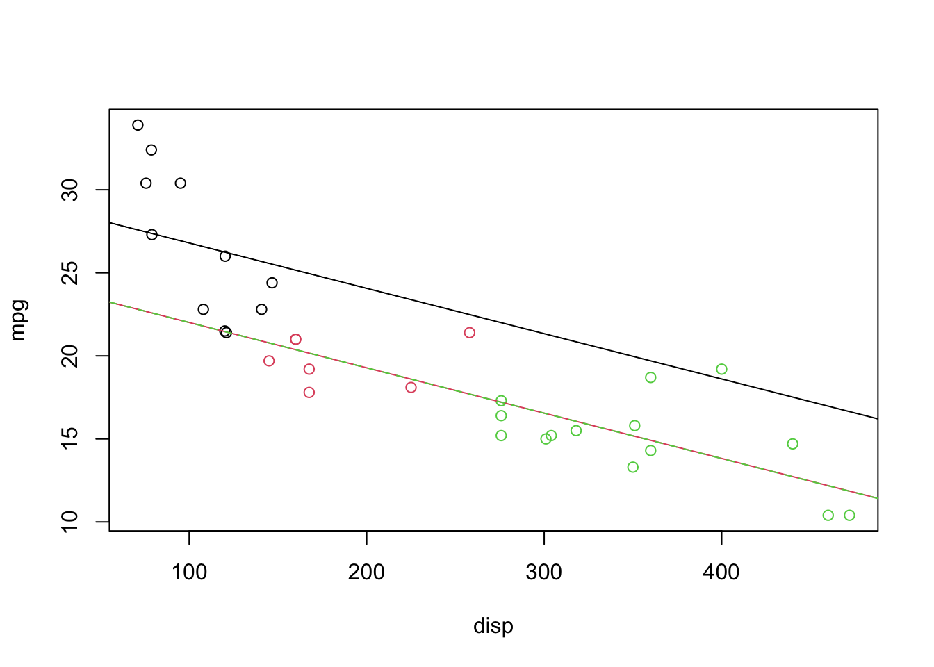
\] This is three different models of mpg versus disp, but with a different intercept depending on the value of cyl.
Show the code
cyldisp <-coef(lm(mpg ~factor(cyl) + disp, data = mtcars))cyldisp
plot(mpg ~ disp, col =factor(cyl), data = mtcars)abline(a = cyldisp[1], b = cyldisp[4], col =1, lty =1)abline(a = cyldisp[1] + cyldisp[2], b = cyldisp[4], col =2, lty =1)abline(a = cyldisp[1] + cyldisp[3], b = cyldisp[4], col =3, lty =2)
The plot looks like it only has 2 lines, but that’s because \(\beta_1=\beta_2\), so one line is plotted on top of the other! I changed the linetypes so you can see this.
It looks like the red and green lines are fitting the red and green data, but the black line doesn’t look quite right.
Three Different Models
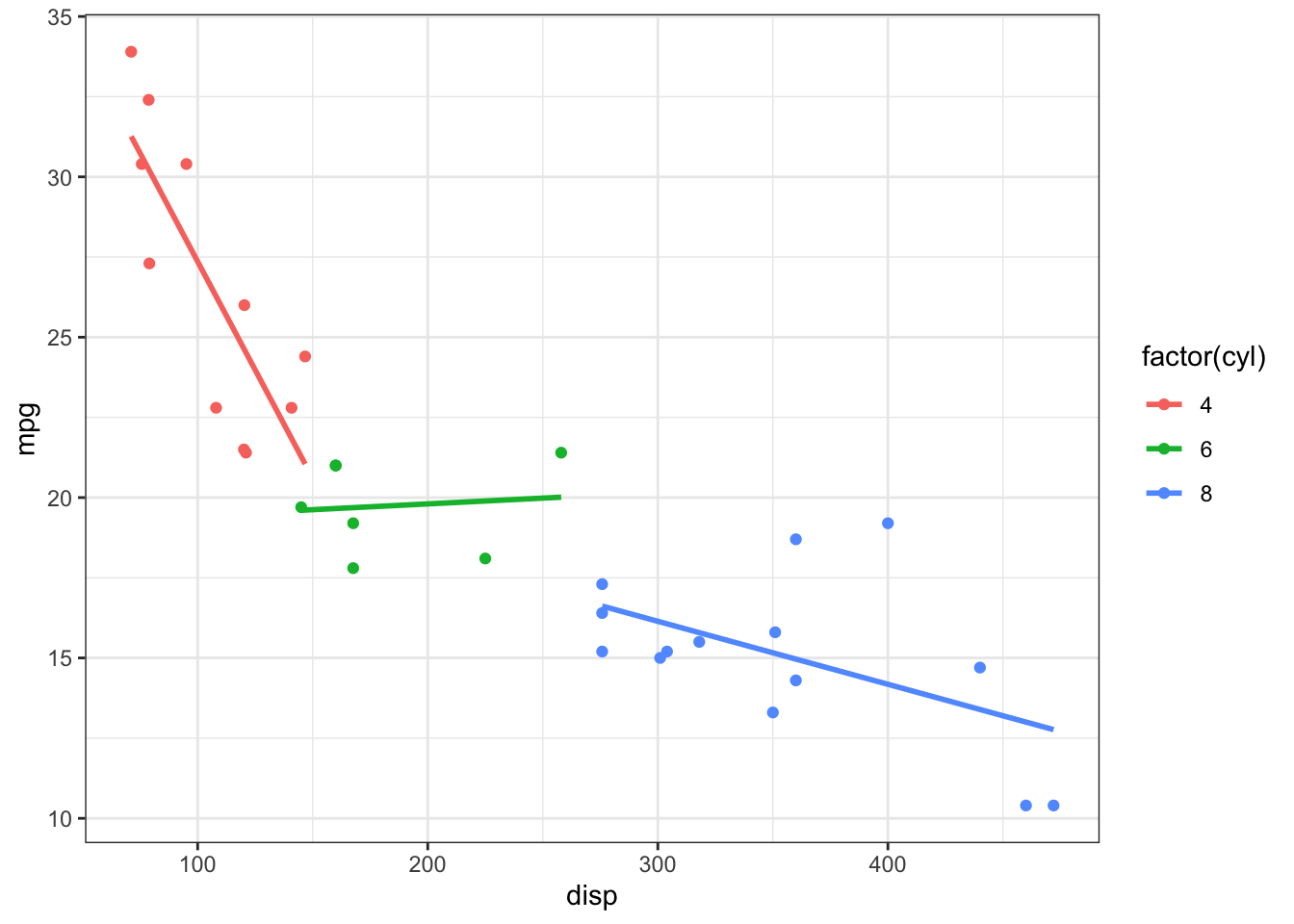
If we have an interaction between cyl and disp, then we essentially get 3 models. \[
y = \beta_0 + \beta_1I(6) + \beta_2I(8) + \beta_3 disp + \beta_4I(6)disp + \beta_5I(8)disp
\] where \(I(6)\) is just shorthand for \(I(cyl == 6)\).
coef(lm(mpg ~ disp, data =subset(mtcars, cyl ==4))) # Others will be similar
(Intercept)        disp
 40.8719553  -0.1351418
ggplot2 makes it super easy to plot this.
Show the code
library(ggplot2); theme_set(theme_bw())ggplot(mtcars) +aes(x = disp, y = mpg, colour =factor(cyl)) +geom_point() +geom_smooth(method ="lm", se =FALSE, formula ="y ~ x")
Recall that the model without interaction terms (different intercepts, same slopes) had practically the same intercept for 6 and 8. The slopes look different here, but there isn’t a lot of data in the 6 category and I suspect that we could force it to have the same intercept and slope as the 8 category.
I.4 Comparison to Other Models
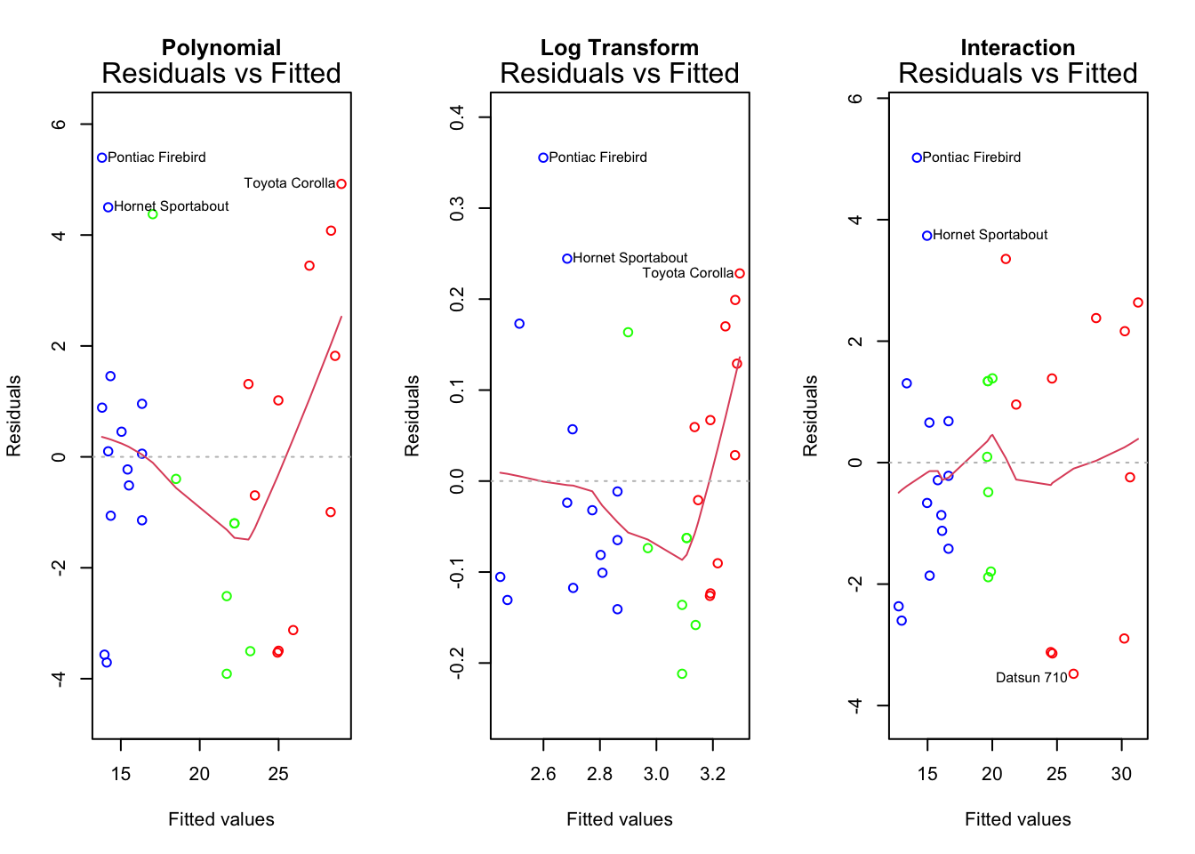
In previous lectures, we’ve looked at this same relationship using polynomial model for displacement and a transformation for mpg. Let’s see how these stack up!
How do we compare such models? There isn’t a statistical test for which one fits best, but, as always, we want to know about the residuals!
Show the code
poly_lm <-lm(mpg ~poly(disp, 2), data = mtcars)log_lm <-lm(log(mpg) ~ disp, data = mtcars)interact_lm <-lm(mpg ~factor(cyl)*disp, data = mtcars)
Show the code
par(mfrow =c(1,3))resid_plot <-1# Re-run with different values to check other plots# Use similar colours to the ggplot.mycolours <-c("red", "green", "blue")[as.numeric(factor(mtcars$cyl))]plot(poly_lm, which = resid_plot, main ="Polynomial", col = mycolours)plot(log_lm, which = resid_plot, main ="Log Transform", col = mycolours)plot(interact_lm, which = resid_plot, main ="Interaction", col = mycolours)
Residuals versus fitted looks quite a bit better for the interaction model.
Normal Q-Q also looks better for interaction model.
Scale-Location is slightly better for interaction model, although still not perfect.
Residuals versus leverage indicates the Hornet 4 Drive car has somewhat high leverage. I’m guessing this is the largest green dot in the plot up above - the green line would be very different without it.
This highlights the importance of carefully interpreting Cook’s Distance. In this case, the interaction model is a combination of three different models.
The plots are quite similar, but for the most part the interaction model seems to work best.
ANOVA can be used to compare the residual variance across non-nested models, but is not appropriate for one of the three models we just saw. See if you can guess which !
Show the code
anova(poly_lm, log_lm, interact_lm)
Analysis of Variance Table

Model 1: mpg ~ poly(disp, 2)
Model 2: mpg ~ factor(cyl) * disp
  Res.Df    RSS Df Sum of Sq      F   Pr(>F)
1     29 233.39
2     26 146.23  3    87.159 5.1655 0.006199 **
---
Signif. codes:  0 '***' 0.001 '**' 0.01 '*' 0.05 '.' 0.1 ' ' 1
The models have a significantly different fit, so the one with the lowest residual variance probably fits better.
The interaction model fits the context of the problem. It absolutely makes sense that an engine with 4 cylinders is different from an engine with 6 cylinders, and part of that difference is the relationship between mpg and displacement. There are no two engines which are equivalent except someone added two cylinders to it; the cylinder values represent fundamentally different groups.
In other words, the theory supports an interaction model. There’s no theory that I know of that states there should be a quadratic relationship between mpg and displacement. If we want to say something about cars in general (inference), it’s best to go with the context of the problem.
The interaction model should fit better since it contains more information - it has the displacement and the number of cylinders, the other models only had displacement.
Also note that the interaction model takes up more degrees of freedom. This can be a negative, especially with small samples.
The p-value for the ANCOVA test is 0.001313, indicating that there is a significantly different covariance between mpg and displacement depending on the number of cylinders.
The lower-order terms factor(cyl) and dispmust be present in order for this test to make sense.
It is technically possible to fit a model with just the interaction term, but it’s slightly better to have extra predictors with a 0 coefficient than be missing predictors with a non-0 coefficient.
For the curious, the syntax for this model would be lm(mpg ~ factor(cyl):disp, data = mtcars), where the : indicates multiplication. This isn’t used often, since it’s almost always incorrect to include interaction terms without the individual effects.
It’s not clearly better in all cases! There may be some contextual reason why it makes sense to only have an interaction.
Recall that the anova() function reports the sequential sum-of-squares. In this situation, we do not care about the p-values for factor(cyl) and disp, so we do not care which order they enter the model in. We only care about the p-value for inclusion of the interaction term factor(cyl):disp.
R’s formula notation is clunky, but leads to a lot of great situations like this. By using factor(cyl)*disp), it added the lower order terms first and then the interaction, thus making the sequential sum-of-squares useful!