Appendix C — Verifying Matrix Identities

Author

Affiliation

Dr. Devan Becker

Wilfrid Laurier University

C.1 Verifying Matrix Results

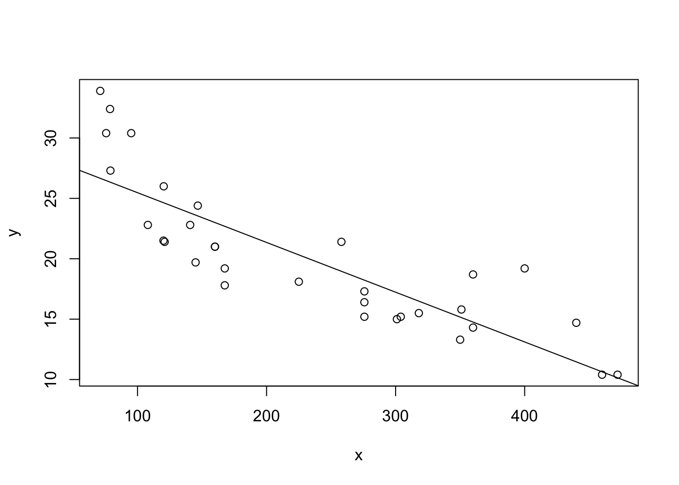
We’ll use the mtcars data for this. Here’s what it looks like:

x <- mtcars$disp
y <- mtcars$mpg

plot(y ~ x)
abline(lm(y ~ x))

It looks like the slope is negative, and the intercept will be somewhere between 25 and 35.

Let’s use the formulae from the previous course: \(\hat\beta_1 = S_{XY}/S_{XX}\) and \(\hat\beta_0 = \bar y - \hat\beta_1\bar x\).

b1 <- sum((x - mean(x)) * (y - mean(y))) / sum((x - mean(x))^2)
b0 <- mean(y) - mean(x) * b1

matrix(c(b0, b1))

            [,1]
[1,] 29.59985476
[2,] -0.04121512

To make the matrix multiplication to work, we need \(X\) to be a column of 1s and a column representing our covariate.

X <- cbind(1, x)
head(X)

         x
[1,] 1 160
[2,] 1 160
[3,] 1 108
[4,] 1 258
[5,] 1 360
[6,] 1 225

The estimates should be \((X^TX)^{-1}X^T\underline y\). In R, we find the transpose with the t() function and we find inverse with the solve() function.

beta_hat <- solve(t(X) %*% X) %*% t(X) %*% y
beta_hat

         [,1]
  29.59985476
x -0.04121512

It works!

Now let’s check the ANOVA table!

n <- length(x)
data.frame(source = c("Regression", "Error", "Total"),
    df = c(2, n-2, n),
    SS = c(t(beta_hat) %*% t(X) %*% y, 
        t(y) %*% y - t(beta_hat) %*% t(X) %*% y,
        t(y) %*% y)
)

      source df         SS
1 Regression  2 13725.1513
2      Error 30   317.1587
3      Total 32 14042.3100

anova(lm(y ~ x))

Analysis of Variance Table

Response: y
          Df Sum Sq Mean Sq F value   Pr(>F)    
x          1 808.89  808.89  76.513 9.38e-10 ***
Residuals 30 317.16   10.57                     
---
Signif. codes:  0 '***' 0.001 '**' 0.01 '*' 0.05 '.' 0.1 ' ' 1

colSums(anova(lm(y ~ x)))

       Df    Sum Sq   Mean Sq   F value    Pr(>F) 
  31.0000 1126.0472  819.4605        NA        NA 

They’re slightly different? Why?

Because the equation in the textbook is for the uncorrected sum of squares, which basically means we’re looking at estimating both \(\beta_0\) and \(\beta_1\) at the same time (hence the df of \(n-2\)). The usual ANOVA table is the corrected sum of squares, which the textbook labels \(SS(\hat\beta_1|\hat\beta_1)\) to make it clear that it’s estimating \(\beta_1\) only; \(\beta_0\) has already been estimated.

n <- length(x)
data.frame(source = c("Regression", "Error", "Total"),
    df = c(1, n-1, n),
    SS = c(t(beta_hat) %*% t(X) %*% y - n * mean(y)^2, 
        t(y) %*% y - t(beta_hat) %*% t(X) %*% y,
        t(y) %*% y - n * mean(y)^2)
)

      source df        SS
1 Regression  1  808.8885
2      Error 31  317.1587
3      Total 32 1126.0472

The matrix form for \(R^2\) is a little different from what you might expect. It uses this idea of “corrected” sum-of-squares as well. For homework, verify that the corrected sum-of-squares works out to the same formula.

Here’s how to extract the \(R^2\) value from R (note that the programming language R has nothing to do with the \(R^2\); R is named after S, which was the programming language that came before it (both chronologically and alphabetically); you’ll still find references to S and S-Plus).

summary(lm(y ~ x))$r.squared

[1] 0.7183433

In the textbook, the formula is given as: \[ R^2 = \frac{\hat{\underline\beta}^TX^T\underline y - n\bar y^2}{\underline y^t\underline y - n\bar y^2} \]

numerator <- t(beta_hat) %*% t(X) %*% y - n * mean(y)^2
denominator <- t(y) %*% y - n * mean(y)^2
numerator / denominator

          [,1]
[1,] 0.7183433

C.2