nrow(peng)[1] 333From last time, we basically learned what the following means:
\[ \frac{SS(\hat\beta_{q+1}, ..., \hat\beta_{p-1} | \hat\beta_0, ... \hat\beta_q)}{(p-q)s^2} =\frac{S_1 - S(\hat\beta_0) - (S_2 - S(\hat\beta_0))}{(p-q)s^2}\sim F_{p-q, \max(p, q)} \] where \(s^2\) is the MSE calculated from the larger model.
This allows us to do a test for whether \(\beta_{q+1} = \beta_{q+2} = ... = \beta_{p-1} = 0\).
Recall that this is accomplished by testing whether the variance of the line significantly changes when those predictors are included. A line with zero variance is horizontal; if adding one predictor to that line changes the variance significantly, then it’s no longer a horizontal line (and thus the slope is non-zero). This works when extending into arbitrary dimensions by adding more predictors - if a predictor is not included in a model, then the hyperplane defined by the linear regression is “horizontal” in that direction.
Mathematically, the regression equation \(y = \beta_0 + \beta_1x_1 + \beta_2x_2\) defines a plane in 3 dimensions, with the slopes determined by \(\beta_1\) and \(\beta_2\) (and a slope of \(1\) in the y direction). If we have also recorded \(x_3\) but not included it in the model, we can write the hyperplane as \(y = \beta_0 + \beta_1x_1 +\beta_2x_2 + 0x_3\), i.e. the hyperplane has a slope of 0 in the \(x_3\) direction. Adding \(x_3\) as a predictor means we are allowing the slope in the \(x_3\) direction to be non-zero.
The big lesson here is that analysing the variance allows us to determine if the slope is 0! This is very important for understanding what’s happening with regression.
The R code to do this test is as follows. In this code, we believe that the bill length and bill depth are strongly correlated, and thus we cannot trust the CIs that we get from summary(lm()) (we saw “Confidence Regions” in the slides and code for L05).
nrow(peng)[1] 333lm1 <- lm(body_mass_g ~ flipper_length_mm + bill_length_mm + bill_depth_mm, data = peng)
lm2 <- lm(body_mass_g ~ flipper_length_mm, data = peng)
anova(lm2, lm1)Analysis of Variance Table
Model 1: body_mass_g ~ flipper_length_mm
Model 2: body_mass_g ~ flipper_length_mm + bill_length_mm + bill_depth_mm
Res.Df RSS Df Sum of Sq F Pr(>F)
1 331 51211963
2 329 50814912 2 397051 1.2853 0.2779Let’s try and calculate these values ourselves in a couple different ways!
anova(lm1)Analysis of Variance Table
Response: body_mass_g
Df Sum Sq Mean Sq F value Pr(>F)
flipper_length_mm 1 164047703 164047703 1062.1232 <2e-16 ***
bill_length_mm 1 140000 140000 0.9064 0.3418
bill_depth_mm 1 257051 257051 1.6643 0.1979
Residuals 329 50814912 154453
---
Signif. codes: 0 '***' 0.001 '**' 0.01 '*' 0.05 '.' 0.1 ' ' 1From this model, SSE is 50814912 on 329 degrees of freedom. This is the same as the SSE in the output of anova(lm2, lm1).
anova(lm2)Analysis of Variance Table
Response: body_mass_g
Df Sum Sq Mean Sq F value Pr(>F)
flipper_length_mm 1 164047703 164047703 1060.3 < 2.2e-16 ***
Residuals 331 51211963 154719
---
Signif. codes: 0 '***' 0.001 '**' 0.01 '*' 0.05 '.' 0.1 ' ' 1Again, the SSE of 51211963 matches what we saw in anova(lm2, lm1), and we have 331 degrees of freedom (as expected, the differences in degrees of freedom is 2).
Note that the F-value in anova() is just the ratio of the MSEs, but this is not the case here. Instead, we need to calculate \(s^2\).
\(s^2\) is the MSE for the larger model:
s2 <- 50814912 / 329
s2
[1] 154452.6And now we can calculate the F-value:
(51211963 - 50814912) / (2 * s2)[1] 1.2853491 - pf(1.28539, 2, 329)[1] 0.2779278anova(lm2, lm1)Analysis of Variance Table
Model 1: body_mass_g ~ flipper_length_mm
Model 2: body_mass_g ~ flipper_length_mm + bill_length_mm + bill_depth_mm
Res.Df RSS Df Sum of Sq F Pr(>F)
1 331 51211963
2 329 50814912 2 397051 1.2853 0.2779There are 3 ways to calculate the ESS for all predictors. They are very helpfully labelled Types I, II, and III.
y ~ x1 + x2 + x1*x2 (although we’ll learn why R uses different notation than this).This will give us every possible sum-of-squares. This is very very dubious, and can lead to a major multiple comparisons problem!
By default, R does sequential sum-of-squares. This is a very important fact to know!
In Types I and II, the order of the predictors matters. In fact, you cannot make any conclusions about the significance that doesn’t make reference to this fact.
## Try changing the order to see how the significance changes!
mylm <- lm(mpg ~ qsec + disp + wt, data = mtcars)
anova(mylm)
Analysis of Variance Table
Response: mpg
Df Sum Sq Mean Sq F value Pr(>F)
qsec 1 197.39 197.39 28.276 1.165e-05 ***
disp 1 615.12 615.12 88.116 3.816e-10 ***
wt 1 118.07 118.07 16.914 0.0003104 ***
Residuals 28 195.46 6.98
---
Signif. codes: 0 '***' 0.001 '**' 0.01 '*' 0.05 '.' 0.1 ' ' 1summary(mylm)$coef # No obvious connection to anova Estimate Std. Error t value Pr(>|t|)
(Intercept) 19.7775575655 5.93828659 3.33051585 0.0024420674
qsec 0.9266492353 0.34209668 2.70873496 0.0113897664
disp -0.0001278962 0.01056025 -0.01211109 0.9904228666
wt -5.0344097167 1.22411993 -4.11267686 0.0003104157\[ y_i = \beta_0 + \beta_1x_i + \beta_2x_i^2 + \beta_3x_i^3 + ... + \beta_{p-1}x_i^{p-1} + \epsilon_i \]
We only have one predictor \(x\), but we have performed non-linear transformations (HMWK: why is it important that the transformations are non-linear?).
What order of polynomial should we fit?
In the code below, I use the I() function (the I means identity) to make the polynomial model. The “formula” notation in R, y ~ x + z, has a lot of options. Including x^2, rather than I(x^2), makes R think we want to do one of the more fancy things, but the I() tells it that we want to literally square it. In the future, we’ll use a better way of doing this.
x <- runif(600, 0, 20)
y <- 2 - 3*x + 3*x^2 - 0.3*x^3 + rnorm(600, 0, 100)
plot(y ~ x)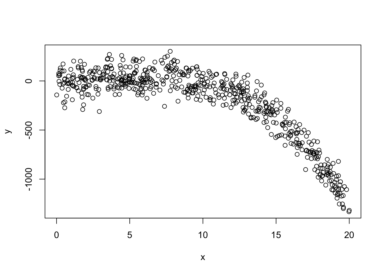
mylm <- lm(y ~ x + I(x^2) + I(x^3) + I(x^4) + I(x^5) + I(x^6))
anova(mylm)
Analysis of Variance Table
Response: y
Df Sum Sq Mean Sq F value Pr(>F)
x 1 49560412 49560412 4726.8201 <2e-16 ***
I(x^2) 1 19661307 19661307 1875.1955 <2e-16 ***
I(x^3) 1 1150679 1150679 109.7459 <2e-16 ***
I(x^4) 1 661 661 0.0630 0.8018
I(x^5) 1 112 112 0.0107 0.9177
I(x^6) 1 6274 6274 0.5984 0.4395
Residuals 593 6217568 10485
---
Signif. codes: 0 '***' 0.001 '**' 0.01 '*' 0.05 '.' 0.1 ' ' 1From the table above, we can clearly see that this should just be a cubic model (which is the true model that we generated). Try changing things around to see if, say, it will still detect an order 5 polynomial if if there’s no terms of order 3 or 4.
Take a moment to consider the following. Suppose I checked the following two (Type II) ANOVA tables:
anova(lm(mpg ~ disp, data = mtcars))anova(lm(mpg ~ disp + wt, data = mtcars))Both tables will have the first row labelled “disp” and include its sum-of-squares along with the F-value. Do you expect these two rows to be exactly the same?
Think about it.
Think a little more.
What values do you expect to be used in the calculation?
Which sums-of-squares? Which variances?
Let’s test it out.
anova(lm(mpg ~ disp, data = mtcars))Analysis of Variance Table
Response: mpg
Df Sum Sq Mean Sq F value Pr(>F)
disp 1 808.89 808.89 76.513 9.38e-10 ***
Residuals 30 317.16 10.57
---
Signif. codes: 0 '***' 0.001 '**' 0.01 '*' 0.05 '.' 0.1 ' ' 1anova(lm(mpg ~ disp + wt, data = mtcars))Analysis of Variance Table
Response: mpg
Df Sum Sq Mean Sq F value Pr(>F)
disp 1 808.89 808.89 95.0929 1.164e-10 ***
wt 1 70.48 70.48 8.2852 0.007431 **
Residuals 29 246.68 8.51
---
Signif. codes: 0 '***' 0.001 '**' 0.01 '*' 0.05 '.' 0.1 ' ' 1They’re different!
With both the polynomial and the disp example, we see that the interpretation of the anova table is highly, extremely, extraordinarily dependent on which predictors we choose to include AND the order in which we choose to include them. So, yeah. Be careful.
There isn’t a built-in function to do this. To create this, we can either use our math (my preferred method) or test each one individually.
anova(
    lm(mpg ~ disp + wt, data = mtcars),
    lm(mpg ~ disp + wt + qsec, data = mtcars)
)
Analysis of Variance Table
Model 1: mpg ~ disp + wt
Model 2: mpg ~ disp + wt + qsec
Res.Df RSS Df Sum of Sq F Pr(>F)
1 29 246.68
2 28 195.46 1 51.22 7.3372 0.01139 *
---
Signif. codes: 0 '***' 0.001 '**' 0.01 '*' 0.05 '.' 0.1 ' ' 1anova(
lm(mpg ~ disp + qsec, data = mtcars),
lm(mpg ~ disp + wt + qsec, data = mtcars)
)Analysis of Variance Table
Model 1: mpg ~ disp + qsec
Model 2: mpg ~ disp + wt + qsec
Res.Df RSS Df Sum of Sq F Pr(>F)
1 29 313.54
2 28 195.46 1 118.07 16.914 0.0003104 ***
---
Signif. codes: 0 '***' 0.001 '**' 0.01 '*' 0.05 '.' 0.1 ' ' 1anova(
lm(mpg ~ wt + qsec, data = mtcars),
lm(mpg ~ disp + wt + qsec, data = mtcars)
)Analysis of Variance Table
Model 1: mpg ~ wt + qsec
Model 2: mpg ~ disp + wt + qsec
Res.Df RSS Df Sum of Sq F Pr(>F)
1 29 195.46
2 28 195.46 1 0.0010239 1e-04 0.9904Minimize the number of p-values that you check.
Minimize the number of degrees of freedom that you use
Suggested textbook Ch06 exercises: E, I, J, N, P, Q, R, X
anova(). Reverse the order of predictors and repeat. Which values in the ANOVA table stay the same? Which values change? Why do they change? What does this tell you about interpreting anova() output?